Regularization for Deep Learning Lecture slides for Chapter 7 of - PowerPoint PPT Presentation

Regularization for Deep Learning Lecture slides for Chapter 7 of Deep Learning www.deeplearningbook.org Ian Goodfellow 2016-09-27

Definition • “Regularization is any modification we make to a learning algorithm that is intended to reduce its generalization error but not its training error.” (Goodfellow 2016)

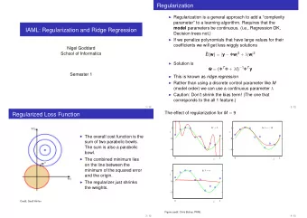
Weight Decay as Constrained Optimization w ∗ ˜ w 2 w w 1 Figure 7.1 (Goodfellow 2016)

Norm Penalties • L1: Encourages sparsity, equivalent to MAP Bayesian estimation with Laplace prior • Squared L2: Encourages small weights, equivalent to MAP Bayesian estimation with Gaussian prior (Goodfellow 2016)

Dataset Augmentation Elastic A ffi ne Noise Deformation Distortion Random Horizontal Translation Hue Shift flip (Goodfellow 2016)

Multi-Task Learning y (1) y (1) y (2) y (2) h (1) h (1) h (2) h (2) h (3) h (3) h (shared) h (shared) x Figure 7.2 (Goodfellow 2016)

Learning Curves Early stopping: terminate while validation set performance is better 0 . 20 Loss (negative log-likelihood) Training set loss Validation set loss 0 . 15 0 . 10 0 . 05 0 . 00 0 50 100 150 200 250 Time (epochs) Figure 7.3 (Goodfellow 2016)

Early Stopping and Weight Decay w ∗ w ∗ ˜ ˜ w 2 w 2 w w w 1 w 1 Figure 7.4 (Goodfellow 2016)

Sparse Representations 2 0 3 2 3 2 3 � 14 3 � 1 2 � 5 4 1 2 6 7 1 4 2 � 3 � 1 1 3 6 7 6 7 6 7 0 6 7 6 7 6 7 19 = � 1 5 4 2 � 3 � 2 6 7 6 7 6 7 0 (7.47) 6 7 6 7 6 7 2 3 1 2 � 3 0 � 3 6 7 4 5 4 5 � 3 4 5 23 � 5 4 � 2 2 � 5 � 1 0 B 2 R m ⇥ n y 2 R m h 2 R n (Goodfellow 2016)

Bagging Original dataset First ensemble member First resampled dataset 8 Second resampled dataset Second ensemble member 8 Figure 7.5 (Goodfellow 2016)

Dropout y y y y Figure 7.6 h 1 h 1 h 2 h 2 h 1 h 1 h 2 h 2 h 1 h 1 h 2 h 2 h 2 h 2 x 1 x 1 x 2 x 2 x 2 x 2 x 1 x 1 x 1 x 1 x 2 x 2 y y y y y h 1 h 1 h 1 h 1 h 2 h 2 h 2 h 2 h 1 h 1 h 2 h 2 x 1 x 1 x 2 x 2 x 1 x 1 x 2 x 2 x 2 x 2 y y y y x 1 x 1 x 2 x 2 h 1 h 1 h 1 h 1 h 2 h 2 Base network x 1 x 1 x 2 x 2 x 1 x 1 x 1 x 1 y y y y h 2 h 2 h 1 h 1 x 2 x 2 (Goodfellow 2016) Ensemble of subnetworks

Adversarial Examples + . 007 ⇥ = x + sign ( r x J ( θ , x , y )) x ✏ sign ( r x J ( θ , x , y )) y = “panda” “nematode” “gibbon” w/ 57.7% w/ 8.2% w/ 99.3 % confidence confidence confidence Figure 7.8 Training on adversarial examples is mostly intended to improve security, but can sometimes provide generic regularization. (Goodfellow 2016)

Tangent Propagation Normal Tangent x 2 x 1 Figure 7.9 (Goodfellow 2016)