Regression Practical Machine Learning Fabian Wauthier 09/10/2009 - PowerPoint PPT Presentation
Regression Practical Machine Learning Fabian Wauthier 09/10/2009 Adapted from slides by Kurt Miller and Romain Thibaux 1 Outline Ordinary Least Squares Regression - Online version - Normal equations - Probabilistic interpretation
Regression Practical Machine Learning Fabian Wauthier 09/10/2009 Adapted from slides by Kurt Miller and Romain Thibaux 1
Outline • Ordinary Least Squares Regression - Online version - Normal equations - Probabilistic interpretation • Overfitting and Regularization • Overview of additional topics - L 1 Regression - Quantile Regression - Generalized linear models - Kernel Regression and Locally Weighted Regression 2
Outline • Ordinary Least Squares Regression - Online version - Normal equations - Probabilistic interpretation • Overfitting and Regularization • Overview of additional topics - L 1 Regression - Quantile Regression - Generalized linear models - Kernel Regression and Locally Weighted Regression 3
Regression vs. Classification: Classification X Y ⇒ Anything: • Discrete: • continuous ( ℜ , ℜ d , …) – {0,1} binary – {1,…k} � multi-class • discrete ({0,1}, {1,…k}, …) – tree, etc. structured • structured (tree, string, …) • … 4
Regression vs. Classification: Classification X Y ⇒ Perceptron Anything: Logistic Regression Support Vector Machine • continuous ( ℜ , ℜ d , …) • discrete ({0,1}, {1,…k}, …) Decision Tree Random Forest • structured (tree, string, …) • … Kernel trick 5
Regression vs. Classification: Regression X Y ⇒ Anything: • continuous: – ℜ , ℜ d • continuous ( ℜ , ℜ d , …) • discrete ({0,1}, {1,…k}, …) • structured (tree, string, …) • … 6
Examples • Voltage Temperature ⇒ • Processes, memory Power consumption ⇒ • Protein structure Energy ⇒ • Robot arm controls Torque at effector ⇒ • Location, industry, past losses Premium ⇒ 7
Linear regression Given examples given a new point Predict y 40 y 26 24 20 22 20 30 40 20 30 20 0 10 0 10 20 10 0 0 x x 8
Linear regression We wish to estimate by a linear function of our data : ˆ x y ˆ = w 0 + w 1 x n +1 , 1 + w 2 x n +1 , 2 y n +1 w ⊤ x n +1 = where is a parameter to be estimated and we have used the w standard convention of letting the first component of be 1. x y 40 y 26 24 20 22 20 30 40 20 30 20 0 10 0 10 20 10 0 0 x x 9
Choosing the regressor Of the many regression fits that approximate the data, which should we choose? Observation � 1 � X i = x i 0 0 20 10 10
LMS Algorithm (Least Mean Squares) In order to clarify what we mean by a good choice of , we will w define a cost function for how well we are doing on the training data: Error or “residual” Observation Prediction � 1 � X i = x i 0 0 20 n 1 Cost = � ( w ⊤ x i − y i ) 2 2 i =1 11
LMS Algorithm (Least Mean Squares) The best choice of is the one that minimizes our cost function w n n E = 1 ( w ⊤ x i − y i ) 2 = � � E i 2 i =1 i =1 In order to optimize this equation, we use standard gradient descent w t +1 := w t − α ∂ ∂wE where n ∂ 1 ∂ ∂ ∂ ∂ w ( w ⊤ x i − y i ) 2 � = ∂ wE i and ∂ wE = ∂ wE i 2 i =1 ( w ⊤ x i − y i ) x i = 12
LMS Algorithm (Least Mean Squares) The LMS algorithm is an online method that performs the following update for each new data point w t − α ∂ w t +1 := ∂ wE i w t + α ( y i − x ⊤ = i w ) x i α∂E i ∂w 13
LMS, Logistic regression, and Perceptron updates • LMS w t + α ( y i − x ⊤ w t +1 := i w ) x i • Logistic Regression w t + α ( y i − f w ( x i )) x i w t +1 := • Perceptron w t + α ( y i − f w ( x i )) x i w t +1 := 14
Ordinary Least Squares (OLS) Error or “residual” Observation Prediction � 1 � X i = x i 0 0 20 n 1 Cost = � ( w ⊤ x i − y i ) 2 2 i =1 15
Minimize the sum squared error n 1 � ( w ⊤ x i − y i ) 2 = E 2 i =1 1 2( Xw − y ) ⊤ ( Xw − y ) = 1 2( w ⊤ X ⊤ Xw − 2 y ⊤ Xw + y ⊤ y ) = ∂ X ⊤ Xw − X ⊤ y ∂ wE = Setting the derivative equal to zero n gives us the Normal Equations X ⊤ Xw X ⊤ y = ( X ⊤ X ) − 1 X ⊤ y = w d 16
A geometric interpretation ∂ ∂wE = X ⊤ ( Xw − y ) = 0 We solved Residuals are orthogonal to columns of X ⇒ gives the best reconstruction of ⇒ y = Xw ˆ y in the range of X 17 17
Residual vector y ! y’ is orthogonal to subspace S y Subspace S spanned by columns of X [X] 2 [X] 1 y’ y’ is an orthogonal 18 projection of y onto S 18
Computing the solution w = ( X ⊤ X ) − 1 X ⊤ y We compute . If X ⊤ X is invertible, then ( X ⊤ X ) − 1 X ⊤ coincides with X + of the pseudoinverse and the solution is unique. X w . If X ⊤ X is not invertible, there is no unique solution w = X + y In that case chooses the solution with smallest Euclidean norm. An alternative way to deal with non-invertible X ⊤ X is to add a small portion of the identity matrix (= Ridge regression). 19 19
Beyond lines and planes Linear models become powerful function approximators when we consider non-linear feature transformations. ⇒ 40 Predictions are still linear in X ! 20 All the math is the same! 0 0 10 20 20
Geometric interpretation y = w 0 + w 1 x + w 2 x 2 ˆ 20 10 400 0 300 200 -10 100 0 10 20 0 [Matlab demo] 21
Ordinary Least Squares [summary] Given examples Let For example Let n d by solving Minimize Predict 22
Probabilistic interpretation 0 0 20 Likelihood 23
25 Conditional Gaussians 20 p(y|x) 15 y Mean µ 10 5 µ =8 µ =3 µ =5 0 0 2 4 6 8 10 24 X 24
BREAK 25
Outline • Ordinary Least Squares Regression - Online version - Normal equations - Probabilistic interpretation • Overfitting and Regularization • Overview of additional topics - L 1 Regression - Quantile Regression - Generalized linear models - Kernel Regression and Locally Weighted Regression 26
Overfitting • So the more features the better? NO! • Carefully selected features can improve model accuracy. • But adding too many can lead to overfitting. • Feature selection will be discussed in a separate lecture. 27 27
Overfitting 30 25 20 Degree 15 polynomial 15 10 5 0 -5 -10 -15 0 2 4 6 8 10 12 14 16 18 20 [Matlab demo] 28
Ridge Regression (Regularization) 15 Effect of regularization (degree 19) Minimize 10 5 with “small” by solving 0 -5 ( X ⊤ X + ǫ I ) w = X ⊤ y -10 0 2 4 6 8 10 12 14 16 18 20 [Continue Matlab demo] 29
Probabilistic interpretation Likelihood Prior Posterior P ( w, x 1 , . . . , x n , y 1 , . . . , y n ) P ( w | X, y ) = P ( x 1 , . . . , x n , y 1 , . . . , y n ) ∝ P ( w.x 1 , . . . , x 1 , y 1 , . . . , y n ) � − 1 � 2 � − ǫ � � � X ⊤ 2 σ 2 || w || 2 � ∝ exp exp i w − y i 2 2 σ 2 i � � �� − 1 � ( X ⊤ ǫ || w || 2 i w − y i ) 2 = exp 2 + 2 σ 2 i 30
Outline • Ordinary Least Squares Regression - Online version - Normal equations - Probabilistic interpretation • Overfitting and Regularization • Overview of additional topics - L 1 Regression - Quantile Regression - Generalized linear models - Kernel Regression and Locally Weighted Regression 31
Errors in Variables (Total Least Squares) 0 0 32
Sensitivity to outliers High weight given to outliers Temperature at noon 25 20 Influence 15 function 10 5 30 40 20 30 20 10 10 0 0 33
L 1 Regression Linear program Influence function [Matlab demo] 34
Quantile Regression ● ● ● ● mean CPU 360 ● ● 95th percentile of CPU ● ● ● ● ● ● ● 340 ● ● ● ● ● ● ● ● ● ● ● CPU utilization [MHz] ● ● ● ● ● ● ● ● ● ● ● ● ● ● ● ● ● 320 ● ● ● ● ● ● ● ● ● ● ● ● ● ● ● ● ● ● ● ● ● ● ● ● ● ● ● ● ● ● ● ● ● ● ● ● ● ● ● ● ● ● ● ● ● ● ● ● ● ● ● ● ● ● 300 ● ● ● ● ● ● ● ● ● ● ● ● ● ● ● ● ● ● ● ● ● ● ● ● ● ● ● ● ● ● ● ● ● ● ● ● ● ● ● ● ● ● ● ● ● ● ● ● ● ● ● ● ● ● ● ● ● ● ● ● ● ● ● ● ● 280 ● ● ● ● ● ● ● ● ● ● ● ● ● ● ● ● ● ● ● ● ● ● ● 260 ● ● ● 15 16 17 18 19 20 21 workload (ViewItem.php) [req/s] Slide courtesy of Peter Bodik 35
Generalized Linear Models Probabilistic interpretation of OLS Mean is linear in X i OLS: linearly predict the mean of a Gaussian conditional. GLM: predict the mean of some other conditional density. f ( X ⊤ � � y i | x i ∼ p i w ) May need to transform linear prediction by to produce a f ( · ) valid parameter. 36 36
Example: “Poisson regression” Suppose data are event counts: y ∈ N 0 y Typical distribution for count data: Poisson Poisson( y | λ ) = e − λ λ y Mean parameter is λ > 0 y ! Say we predict λ = f ( x ⊤ w ) = exp x ⊤ w � � f ( X ⊤ � � y i | x i ∼ Poisson i w ) GLM: 37 37
Recommend
More recommend
Explore More Topics
Stay informed with curated content and fresh updates.
