Notes on Linear Least Squares Model, COMP24111 Tingting Mu - PDF document

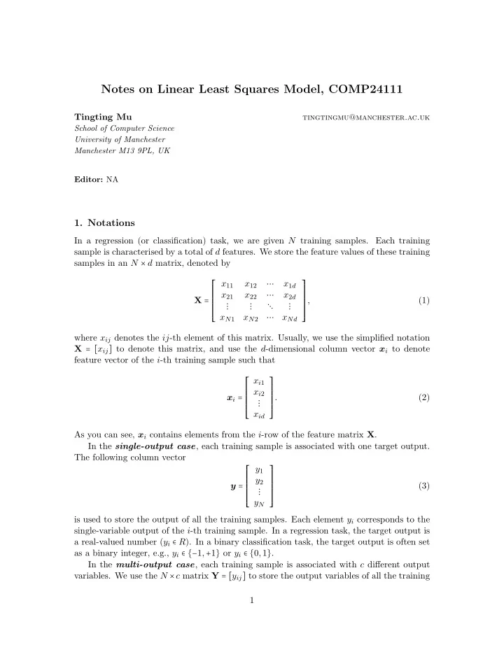
Notes on Linear Least Squares Model, COMP24111 Tingting Mu tingtingmu@manchester.ac.uk School of Computer Science University of Manchester Manchester M13 9PL, UK Editor: NA 1. Notations In a regression (or classification) task, we are given N training samples. Each training sample is characterised by a total of d features. We store the feature values of these training samples in an N × d matrix, denoted by ⎡ ⎤ ⋯ ⎢ ⎥ ⎢ x 11 x 12 x 1 d ⎥ ⋯ ⎢ ⎥ X = ⎢ ⎥ x 21 x 22 x 2 d ⎢ ⎥ ⋮ ⋮ ⋱ ⋮ , (1) ⎢ ⎥ ⎢ ⎥ ⋯ ⎣ ⎦ x N 1 x N 2 x Nd where x ij denotes the ij -th element of this matrix. Usually, we use the simplified notation X = [ x ij ] to denote this matrix, and use the d -dimensional column vector x i to denote feature vector of the i -th training sample such that ⎡ ⎤ ⎢ ⎥ ⎢ x i 1 ⎥ ⎢ ⎥ x i = ⎢ ⎥ x i 2 ⎢ ⎥ ⋮ . (2) ⎢ ⎥ ⎢ ⎥ ⎣ ⎦ x id As you can see, x i contains elements from the i -row of the feature matrix X . In the single-output case , each training sample is associated with one target output. The following column vector ⎡ ⎤ ⎢ ⎥ ⎢ y 1 ⎥ ⎢ ⎥ y = ⎢ ⎥ y 2 ⎢ ⎥ ⋮ (3) ⎢ ⎥ ⎢ ⎥ ⎣ ⎦ y N is used to store the output of all the training samples. Each element y i corresponds to the single-variable output of the i -th training sample. In a regression task, the target output is a real-valued number ( y i ∈ R ). In a binary classification task, the target output is often set as a binary integer, e.g., y i ∈ { − 1 , + 1 } or y i ∈ { 0 , 1 } . In the multi-output case , each training sample is associated with c different output variables. We use the N × c matrix Y = [ y ij ] to store the output variables of all the training 1

samples: ⎡ ⎤ ⋯ ⎢ ⎥ ⎢ y 11 y 12 y 1 c ⎥ ⋯ ⎢ ⎥ Y = ⎢ ⎥ y 21 y 22 y 2 c ⎢ ⎥ ⋮ ⋮ ⋱ ⋮ . (4) ⎢ ⎥ ⎢ ⎥ ⋯ ⎣ ⎦ y N 1 y N 2 y Nc We use the c -dimensional column vector ⎡ ⎤ ⎢ ⎥ ⎢ y i 1 ⎥ ⎢ ⎥ y i = ⎢ ⎥ y i 2 ⎢ ⎥ ⋮ (5) ⎢ ⎥ ⎢ ⎥ ⎣ ⎦ y ic to store the c output variables of the i -th training sample. 2. Linear Model In machine learning, building a linear model refers to employing a linear function to estimate a desired output. The general formulation of a linear function that takes n input variables is f ( x 1 ,x 2 ,...,x n ) = a 0 + a 1 x 1 + a 2 x 2 + ⋯ a n x n , (6) where a 0 ,a 1 ,a 2 ...a n are often referred to as the linear combination coefficients (weights), or linear model weights. 2.1 Single-output Case We use one linear function to estimate the single output variable of a given sample based on its input features x = [ x 1 ,x 2 ,...,x d ] T . The estimated output is given by y = w 0 + w 1 x 1 + w 2 x 2 + ⋯ w d x d = w 0 + d w i x i = w T ˜ ∑ ˆ x , (7) i = 1 where the column vector w = [ w 0 ,w 1 ,w 2 ,...,w d ] T stores the model weights. The modified notation ⎡ ⎤ ⎢ ⎥ 1 ⎢ ⎥ ⎢ ⎥ ⎢ ⎥ x 1 x = ⎢ ⎥ ⎢ ⎥ ˜ x 2 (8) ⎢ ⎥ ⋮ ⎢ ⎥ ⎢ ⎥ ⎣ ⎦ x d is introduced to simplify the writing of the linear model formulation, and it is called the expanded feature vector. 2

2.2 Multi-output Case In this case, each target output is estimated using one linear function. We seek c different functions to predict the c output for a sample x = [ x 1 ,x 2 ,...,x d ] T : = w 01 + w 11 x 1 + w 21 x 2 + ⋯ w d 1 x d = w T ˆ 1 ˜ (9) y 1 x , = w 02 + w 12 x 1 + w 22 x 2 + ⋯ w d 2 x d = w T y 2 ˆ 2 ˜ x , (10) ⋮ = w 0 c + w 1 c x 1 + w 2 c x 2 + ⋯ w dc x d = w T y c ˆ c ˜ x , (11) where the vector ⎡ ⎤ ⎢ ⎥ w 0 i ⎢ ⎥ ⎢ ⎥ ⎢ ⎥ w 1 i w i = ⎢ ⎥ ⎢ ⎥ (12) w 2 i ⎢ ⎥ ⋮ ⎢ ⎥ ⎢ ⎥ ⎣ ⎦ w di stores the linear model weights for predicting the i -th target output. By collecting all the estimated output in a vector, a neat expression of the multi-output linear model can be obtained: ⎡ ⎤ ⎡ ⎤ ⎡ ⎤ ⎡ ⎤ w 01 + w 11 x 1 + w 21 x 2 + ⋯ w d 1 x d ⎢ ⎥ ⎢ ⎥ ⎢ ⎥ ⎢ ⎥ ⎢ y 1 ˆ ⎥ ⎢ ⎥ ⎢ w 01 w 11 w 21 ... w d 1 ⎥ ⎢ 1 ⎥ w 02 + w 12 x 1 + w 22 x 2 + ⋯ w d 2 x d ⎢ ⎥ ⎢ ⎥ ⎢ ⎥ ⎢ ⎥ y = ⎢ ⎥ = ⎢ ⎥ = ⎢ ⎥ ⎢ ⎥ = W T ˜ y 2 ˆ w 02 w 12 w 22 ... w d 2 x 1 ⎢ ⎥ ⎢ ⎥ ⎢ ⎥ ⎢ ⎥ ⋮ ⋮ ⋮ ⋮ ⋮ ⋱ ⋮ ⋮ ˆ x , ⎢ ⎥ ⎢ ⎥ ⎢ ⎥ ⎢ ⎥ ⎢ ⎥ ⎢ ⎥ ⎢ ⎥ ⎢ ⎥ w 0 c + w 1 c x 1 + w 2 c x 2 + ⋯ w dc x d ⎣ ⎦ ⎣ ⎦ ⎣ ⎦ ⎣ ⎦ y c ˆ w 0 c w 1 c w 2 c ... w dc x d (13) where the ( d + 1 ) × c matrix ⎡ ⎤ ⋯ ⎢ ⎥ w 01 w 02 w 0 c ⎢ ⎥ ⋯ ⎢ ⎥ ⎢ ⎥ w 11 w 12 w 1 c W = ⎢ ⋯ ⎥ ⎢ ⎥ w 21 w 22 w 2 c . (14) ⎢ ⎥ ⋮ ⋮ ⋱ ⋮ ⎢ ⎥ ⎢ ⎥ ⋯ ⎣ ⎦ w d 1 w d 2 w dc stores all the model weights. 3. Least Squares Training a linear model refers to the process of finding the optimal values of the model weights, by utilising information provided by the training samples. The least squares ap- proach refers to the method of finding the optimal model weights by minimising the sum- of-squares error function. 3.1 Sum-of-squares Error The sum-of-squares error function is computed as the sum of the squared differences between the true target outputs and their estimation. In the single-output case, the error function computed using N training samples is given as y i − y i ) 2 = 2 O ( w ) = N ( ˆ N (( w 0 + d w k x ik ) − y i ) = N ( w T ˜ x i − y i ) ∑ ∑ ∑ ∑ 2 , (15) i = 1 i = 1 k = 1 i = 1 3

x i = [ 1 ,x i 1 ,x i 2 ,...x id ] T is the expanded feature vector for the i -th training sample. where ˜ In the multi-output case, each sample is associated with multiple output variables (e.g., y i 1 ,y i 2 ,...,y ic for the i -th training sample). The error function is computed by examining the squared difference over each target output of each training sample, resulting in the following sum: y ij − y ij ) 2 = 2 N c N c d N c O ( W ) = ( ˆ (( w 0 j + w kj x ik ) − y ij ) = ( w T x i − y ij ) ∑ ∑ ∑ ∑ ∑ ∑ ∑ 2 . j ˜ (16) i = 1 j = 1 i = 1 j = 1 k = 1 i = 1 j = 1 3.2 Normal Equations Normal equations provide a way to find the model weights that minimises the sum-of- squares error function. It is derived by setting the partial derivatives of the error function with respect to the weights to zero. We first look at the single-output case, and use w ∗ to denote the optimal weight vector that minimises the sum-of-squares error function. The normal equations are w ∗ = ( ˜ − 1 ˜ X ) T y = ˜ T ˜ + y , (17) X X X ⎡ ⎤ where ⋯ ⎢ ⎥ 1 ⎢ x 11 x 12 x 1 d ⎥ ⋯ ⎢ ⎥ X = ⎢ ⎥ 1 x 21 x 22 x 2 d ˜ ⎢ ⎥ ⋮ ⋮ ⋮ ⋱ ⋮ (18) ⎢ ⎥ ⎢ ⎥ ⋯ ⎣ ⎦ 1 x N 1 x N 2 x Nd + = ( ˜ − 1 ˜ X ) T ˜ T is called the Moore- The quantity ˜ is the expanded feature matrix. X X X Penrose pseudo-inverse of the matrix. To compute the optimal weight matrix W ∗ for the multi-output case, the normal equa- tions possess a similar form to Eq. (17): W ∗ = ( ˜ − 1 ˜ X ) T Y = ˜ T ˜ + Y . (19) X X X When implementing the normal equations, you can seek help from existing linear algebra libraries, e.g. “inv()”, “pinv()” in MATLAB, to compute the inverse or pseudo-inverse of a given matrix. If you are interested in how to derive the normal equations, you can read the optional reading materials in Section 4. 3.3 Regularised Least Squares model The regularised least squares model finds its model weights by minimising the following modified error function: y i − y i ) 2 + λ ( w 2 O ( w ) = N ( ˆ 0 + d i ) ∑ ∑ w 2 (20) i = 1 i = 1 for the single-output case, and y ij − y ij ) 2 + λ O ( W ) = N c ( ˆ c ( w 2 0 j + d ij ) ∑ ∑ ∑ ∑ w 2 (21) i = 1 j = 1 j = 1 i = 1 4