Regression Models Response Variable (Y). Explanatory (or predictor) - - PowerPoint PPT Presentation

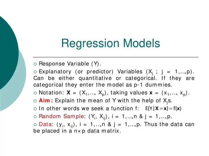
Regression Models

 Response Variable (Y).  Explanatory (or predictor) Variables (Xj ; j =

1,… ,p). Can be either quantitative or categorical. If they are categorical they enter the model as p-1 dummies.

 Notation: X = (X1,…

, Xp), taking values x = (x1,… , xp).

 Aim : Explain the mean of Y with the help of Xjs.  In other words we seek a function f:  Random Sample: (Yi, Xij), i = 1,…

,n & j = 1,… ,p.

 Data: (yi, xij), i = 1,…

,n & j = 1,… ,p. Thus the data can be placed in a n× p data matrix.

= = E(Y| ) f( ) X x x

Normal Linear Regression Model



Let Y be quantitative taking values in the whole real line.



For simplicity we assume that f is a linear function.



We assume that (Y| X= x) follows a normal distribution with constant (unknown) variance. Thus:



Therefore



Similarly we can write



The above representation (with the error term) is only valid in normal regression models.



Thus our model is random and not deterministic.



The quantity is called the systematic component.



The parameters β = (β0,….,βp) & σ2 are unknown and we estimate them using the available data.



Once we estimate them we can estimate the conditional mean of Y using the systematic companent.

2 1 1 p p

(Y | ) N( x ... x , ) = ∼ β + β + + β σ X x

2 1 1 p p

Y x ... x , ~ (0, ) = β + β + + β + ε ε Ν σ

1 1 p p

E(Y | ) x ... x = = β + β + + β X x

1 1 p p

n x ... x = β + β + + β

Binary Regression Model



Let Y be binary taking values 0 (failure) or 1 (success). Then Y ~ Bernoulli(p), with p = P(Y= 1) = E(Y).



Therefore in this case the mean of the response variable takes values in (0,1).



On the other hand the systematic component in general takes values in the whole real line!



Thus if we write as before we have a problem! We equate the left quantity that takes values in (0,1) with the right quantity that takes values on the whole real line. Thus we might end up estimating the probability of success of Y with a value above 1 or below zero!



How to solve the problem? We can introduce a function g, that we call it link function, that transforms, e.g. the left hand side of the above equation to take values in the whole real line.



Thus g(p): (0,1) -> (-∞,+∞) and we write

1 1 p p

E(Y | ) P(Y 1| ) x ... x = ≡ = = = β + β + + β X x X x

[ ]

1 1 p p

g E(Y | ) x ... x = = β + β + + β X x

Binary Regression Model

 Many such functions g exist.  Examples:

 Logit  Probit  Complementary Log-Log

 The logit function has a very simple

a nice interpretation!

Binary Logistic Regression



Let’s denote by p = E(Y| X= x).



Remember that this is the probability of “success” of Y when X =

• x. Then 1-p is the probability of “failure” of Y when X = x.



We call odds the quantity



Interpretation: It provides the number we need to multiply the probability

• f

failure in

• rder

to calculate the probability

• f

success. For example

• dds

= 2 implies that the success probability is twice as high as the failure probability, while odds = 0.6 implies that the success probability is equal to 60% the failure probability. The quantity (odds-1)100% provides the percentage increase or decrease (depending on the sign) of the success probability in comparison to the failure probability. For example odds = 1.6 indicates that the success probability is 60% higher that the corresponding failure probability, while odds = 0.6 indicates that the success probability is 40% lower that the corresponding failure probability.



If additionally we take logs (natural) we have

p

• dds
• dds(Y

1) (0, ) 1 p ≡ = = ∈ +∞ − p log(odds) log ( , ) 1 p   = ∈ −∞ +∞   −  

Binary Logistic Regression

1 1 p p 1 p 1 1 p p

exp( X X ) P(Y 1| X , ,X ) 1 exp( X X ) β +β + +β

• =

= + β +β + +β   

1 1 p p 1 p 1 1 p p 1 1 p p

exp( X X ) P(Y 0 | X , ,X ) 1 1 exp( X X ) 1 1 exp( X X ) β +β + +β

• =

= − + β +β + +β = + β +β + +β    

1 p 1 1 p p 1 p

P(Y 1| X , ,X ) exp( X X ) P(Y 0 | X , ,X ) =

• =

β +β + +β =   

1 p 1 1 p p 1 p

P(Y 1| X , ,X ) Log X X P(Y 0 | X , ,X )   =

• = β +β

+ +β     =     

Logistic Function

Binary Logistic Regression

 Note that this logistic function is

S-shaped, which means that changing the exposure level does not affect the probability much if the exposure level is low

• r high.

Binary Logistic Regression

0,0 0,2 0,4 0,6 0,8 1,0

x x

e P("Success"| x) 1 e

α+β α+β

= + x P(“Success”| x)

E.g. buying a new car E.g. salary

Binary Logistic Regression

 Equivalently, a Logistic Regression Model

is to model the logarithm of the conditional odds of Y= 1 given explanatory variables X1,… ,Xp as a linear function of X1,… ,Xp , i.e.,

1 p 1 1 p p

Log odds(Y 1| X , ,X ) X X   = = α + β + + β     Good News! We are back to a linear function!

Odds Ratio

 The ratio of two odds of two different outcomes

are called

• dds

ratios (OR) and provide the relative change of the odds under two different conditions (for example X = 1, 2).

 When OR21 = 1, then the conditional odds under

comparison are equal, indicating no difference in the relative success probability of Y under X = 1 & X = 2. The quantity (OR21 - 1)100% provides the percentage change of the odds for X = 2 compared with the corresponding odds when X = 1.

21

• dds(Y

1| X 2) OR

• dds(Y

1| X 1) = = = = =

conditional odds

Odds Ratio

 Interpretation:



β0: The odds of Y = 1 when all Xs are 0 is exp(β0).



βj: The ratio of the odds (odds ratio) of Y= 1 for Χj= xjo+ 1 to the odds of Y= 1 for Χj= xjo, when all other explanatory variables are held constant is exp(βj).



For example if exp(βj) = 1.17 we can say for a one-unit increase in Xj (and keeping other variables fixed), we expect to see about 17% increase in the odds of Y= 1. This 17% of increase does not depend on the value that Xj is held at (xjo).



Similarly if exp(βj) = 0.90 we can say for a one-unit increase in Xj (and keeping other variables fixed), we expect to see about 10% decrease in the odds of Y= 1. This 10% of decrease does not depend on the value that Xj is held at (xjo).



If Xj is dummy, exp(βj) represents the ratio of the odds of Y= 1 when the corresponding categorical variable takes the level denoting by Xj = 1 to the odds of Y= 1 when the categorical variable takes the value of the reference category (the one without dummy), keeping all other explanatory variables fixed.

Other Link functions g for Binary Regression

 Probit: Φ-1(p), Φ is the cdf of N(0,1).  Complementary Log-Log:

log(-log(1-p)), log is the natural logarithm.

Other Link functions g for Binary Regression

Binomial Regression Model

 Let Y ~ Binomial(N, p), with N known.  Again we model p, and thus the same

approach is used as before in the Binary Regression Models.

 Most common model is again here the

logistic regression one, due to the nice interpretations that provides.

Poisson Regression Model



Let Y ~ Poisson(λ), λ > 0.



Then E(Y) = λ > 0.



Thus in this case we need a link function g(λ): (0, +∞) -> (-∞,+∞) and we write



Most common choice is the log function (natural logarithm).



If the predictor is quantitative, then for a one unit change in the predictor variable, the difference in the logs of expected value of Y is expected to change by the respective regression coefficient, given the other predictor variables in the model are held constant.



If the predictor is dummy, then the we interpret the coefficient as

• follows. When the corresponding categorical variable from the value
• f the reference category level takes the level denoting by Xj = 1,

then the difference in the logs of expected value of Y is expected to change by the respective regression coefficient, given the other predictor variables in the model are held constant.

[ ]

1 1 p p

g E(Y | ) x ... x = = β + β + + β X x

Generalized Linear Model

 All the previous examples belong in

the area of Generalized Linear Models (GLMs).

 Many more…

..

 E.g. Gamma, Negative Binomial,

etc.

 The distribution should be a

member of the exponential family.