Machine Learning Lecture 4 Justin Pearson 1 2020 1 - PowerPoint PPT Presentation
Machine Learning Lecture 4 Justin Pearson 1 2020 1 http://user.it.uu.se/~justin/Teaching/MachineLearning/index.html 1 / 42 Todays plan Very quick Revision on Linear Regression. Logistic Regression Another classification algorithm More
Machine Learning Lecture 4 Justin Pearson 1 2020 1 http://user.it.uu.se/~justin/Teaching/MachineLearning/index.html 1 / 42
Today’s plan Very quick Revision on Linear Regression. Logistic Regression — Another classification algorithm More on confusion matrices and F-scores. 2 / 42
Classification and Regression Remember two fundamental different learning tasks Regression From input data predict and or learn a numeric value. Classification From the input data predict or learn what class a class something falls into. More lingo from statistics. A variable is Categorical if it can take one of a finite number of discrete values. 3 / 42
Linear Regression Given m data samples x = ( x (1) , . . . , x ( m ) ) and y = ( y (1) , . . . , y ( m ) ). We want to find θ 0 and theta θ 1 such that J ( θ 0 , θ 1 , x , y ) is minimised. That is we want to minimise m J ( θ 0 , θ 1 , x , y ) = 1 � ( h θ 0 ,θ 1 ( x ( i ) ) − y ( i ) ) 2 2 m i =1 Where h θ 0 ,θ 1 = θ 0 + θ 1 x 4 / 42
Linear Regression — Partial Derivatives m J ( θ ) = 1 ∂ � ( h θ 0 ( x ( i ) ) − y ( i ) ) ∂θ 0 m i =1 m J ( θ ) = 1 ∂ ( h θ 0 ,θ 1 ( x ( i ) ) − y ( i ) ) x ( i ) � j ∂θ j m i =1 For linear regression you can either find an exact solution minimising J ( θ ) by setting the partial derivatives to zero or using gradient descent. 1 , . . . , x ( ) To avoid treating θ 0 as a special case transform your data ( x ( i ) n i ) 1 , . . . , x ( ) to (1 , x ( i ) n i ) ( x ( i ) = 1). 0 5 / 42
L 2 Regularisation To avoid over fitting we sometimes want to stop the coefficients to large. m n J ( θ ) = 1 ( h θ ( x ( i ) ) − y ( i ) ) 2 + λ � � θ 2 i 2 m i =1 i =1 There is an exact solution or you can use gradient descent. 6 / 42
L 1 Regularisation m n J ( θ ) = 1 ( h θ ( x ( i ) ) − y ( i ) ) 2 + λ � � | θ i | 2 m i =1 i =1 Where |·| is the absolute value function. This has no analytic solution. You have to use gradient descent or some other optimisation algorithm. 7 / 42
How do you select your model? We saw that there are a lot of choices of what model you can choose. You can fit higher order polynomials. You can have non-linear features such x i x j where x i could be for example the width and x j could be the breadth and x i x j would represent an area. You can reduce the number of features. Picking features is quite complex and we will look at it later. There is also a bigger question, if you have a number of different models how do you decide which to pick? We will look at cross-validation later as well. 8 / 42
Classification and Regression Remember two fundamental different learning tasks Regression From input data predict and or learn a numeric value. Classification From the input data predict or learn what class a class something falls into. More lingo from statistics. A variable is Categorical if it can take one of a finite number of discrete values. 9 / 42
Classification General problem of classification. 7.5 5.0 2.5 0.0 2.5 5.0 7.5 10.0 2 0 2 4 6 8 10 Given a number of classes find a way to separate them. 10 / 42
Approaches to Classification Probabilistic Classification Try to predicate the probability that an put sample x belongs to a class: P ( C | x ). Learn a hypothesis h θ such that h θ ( x ) = 1 if x belongs to the class and h θ ( x ) = 0 otherwise. With Naive Bayes we calculated P ( C | x ) by looking at P ( x | C ) P ( C ). Instead we could try to estimate P ( C | x ) directly. 11 / 42
Hypotheses for Classification Learning (and even formulating) hypothesises h θ such that h θ ( x ) = 1 if x belongs to the class and h θ ( x ) = 0 otherwise is quite hard. It is better to use threshold values and learn an hypotheses such that � 1 if h θ ( x ) ≤ 0 . 5 C θ ( x ) = 0 if h θ ( x ) > 0 . 5 12 / 42
Hypotheses for Classification For the one dimensional case we want to learn some sort of step function � 1 if θ 0 + θ 1 x > 0 . 5 h θ 0 ,θ 1 = 0 if θ 0 + θ 1 x ≤ 0 . 5 1.0 0.8 0.6 0.4 0.2 0.0 0 2 4 6 8 10 12 In general it will be very hard find values of θ 0 and θ 1 that minimise the error on our training set. Gradient descent will not work, and there is no easy exact solution. 13 / 42
The Logistic-Sigmoid Function Two(ish) approaches to get (Logisitic)-sigmoid functions Try to approximate step functions with a continuous function. An argument from probability with log odds ratio. Biological motivation neurons and activation functions: Modelling the firing rate of neurons 14 / 42
The Logistic-Sigmoid Function 1 σ ( x ) = 1 + e − x 1.0 0.8 0.6 0.4 0.2 0.0 10.0 7.5 5.0 2.5 0.0 2.5 5.0 7.5 10.0 15 / 42
The Logistic-Sigmoid Function In general we combine it with a linear function 1 h θ 0 ,θ 1 ( x ) = 1 + e − θ 1 x + θ 0 As θ 1 gets larger the function looks more a step function. 1.0 0.5 1 2 0.8 0.6 0.4 0.2 0.0 10.0 7.5 5.0 2.5 0.0 2.5 5.0 7.5 10.0 16 / 42
The Logistic-Sigmoid Function — an informal interpretation Since for 1 h θ 0 ,θ 1 ( x ) = 1 + e − θ 1 x + θ 0 we have that 0 ≤ h ( x ) ≤ 1 We could interpret h ( x ) is a probability that x belongs to a class. 17 / 42
Derivative of the Sigmoid function The sigmoid function 1 σ ( x ) = 1 + e − x Has a rather nice derivative σ ′ ( x ) = σ ( x )(1 − σ ( x )) 18 / 42
Gradient Descent Since we can take the derivative sigmoid function it is possible to calculate the partial derivatives of the cost function m J ( θ, x , y ) = 1 � ( σ ( θ T x ( i ) ) − y ( i ) ) 2 2 m i =1 Where θ is a vector of values. 19 / 42
Neural Networks — Very Briefly — Not examined A single (artificial) neuron can be modelled as 1 h w 1 ,..., w k ,θ 0 ( x 1 , . . . , x k ) = 1 + exp( � k i =1 w i x i + θ 0 ) For a single neuron apply gradient descent to the function m J ( w 1 , . . . , w k , θ 0 ) = 1 � ( h w 1 ,..., w k ,θ 0 ( x ( i ) ) − y ( i ) ) 2 2 m i =1 For multiple layer neural networks you just keep applying the chain rule and you get back-propagation. 20 / 42
Neural Networks — Very Briefly — Not examined Allow you to do very powerful non-linear regression. Even though the cost function is highly non-linear it is generally possible minimise the error. Very sensitive to the architecture: the number of layers, how many neurons in each layer. For very large networks you need a lot of data to learn the weights. Often you get vanishing gradients. That is for some weight w the quantity ∂ J ∂ w can be very small. This can make convergence very slow. Since tuning neural networks can be hard, try other methods first. With deep learning when they work they work, when they do not work nobody really knows why. 21 / 42
Odds Ratio Given an event with probability p we can take the odds ratio of p happening and p not happening. p 1 − p 22 / 42
Log Odds Ratio For various reasons it is better to study � � p log 1 − p Log-Odds make non-linear things slightly more linear and more symmetric. 23 / 42
Log Odds classifier If we use log-odds we are interested in the quantity P ( C | x ) the probability that we are in the class C given the data x . If we look at the log-odds ratio and use a linear classifier h θ ( x ) = � m i =1 θ i x i + θ 0 . � P ( C | x ) � � P ( C | x ) � log = log = h θ ( x ) 1 − P ( C | x ) P ( C | x ) A bit of algebra � P ( C | x ) � � � P ( C | x ) = = exp( h θ ( x )) 1 − P ( C | x ) P ( C | x ) 24 / 42
More algebra � P ( C | x ) � = exp( h θ ( x )) 1 − P ( C | x ) Gives P ( C | x ) = exp( h θ ( x ))(1 − P ( C | x )) Thus with a bit more algebra we can get exp( h θ ( x )) 1 P ( C | x ) = 1 + exp( h θ ( x )) = 1 + exp( − h θ ( x )) 25 / 42
Logistic regression Thus if 1 P ( C | x ) = 1 + exp( − h θ ( x )) We are modelling the log-odds ratio, which is a good thing. 26 / 42
Cross Entropy Cost The standard cost/loss/error function m J ( θ ) = 1 � ( σ ( h θ ( x ( i ) )) − y ( i ) ) 2 2 m i =1 Is not really suitable if the expected values y ( i ) can only be 0 or 1. We really want to count the number of miss-classifications. We would also like something convex (one minimum as in linear regression) 27 / 42
Cross Entropy Cost � − log( σ ( h θ ( x ))) if y = 1 Cost θ ( x ) = − log(1 − σ ( h θ ( x ))) if y = 0 There are lots of ways of motivating this. One it to use information theory, another is via maximum likelihood estimation. Most importantly (although the proof is outside the scope of the course) it is concave and hence gradient descent will converge to the global minimum. 28 / 42
Cross Entropy Cost — Intuitive Picture � − log( σ ( h θ ( x ))) if y = 1 Cost θ ( x ) = − log(1 − σ ( h θ ( x ))) if y = 0 Suppose our target value y is equal to 1, and σ ( h θ ( x )) is close to 1 then Cost θ ( x ) will be close to 0. Remember log (1) = 0. Again when y = 1 if when σ ( h θ ( x )) gets closer to 0 then − log( σ ( h θ ( x ))) gets larger and larger. We heavily penalise values away from 1. 29 / 42
Recommend
More recommend
Explore More Topics
Stay informed with curated content and fresh updates.


