Regression: Choosing Variables LIR 832 November 14, 2006 Topics of - - PDF document

1

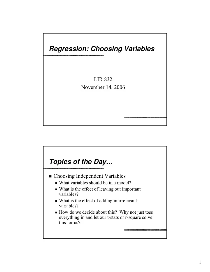
Regression: Choosing Variables

LIR 832 November 14, 2006

Topics of the Day…

Choosing Independent Variables

What variables should be in a model? What is the effect of leaving out important

variables?

What is the effect of adding in irrelevant

variables?

How do we decide about this? Why not just toss

everything in and let our t-stats or r-square solve this for us?

2

Example: Effect of Unions (x) on Weekly Earnings (y)

reg lnwage cbc2 Source | SS df MS Number of obs = 156130

• ------------+------------------------------

F( 1,156128) = 3897.11 Model | 1234.14281 1 1234.14281 Prob > F = 0.0000 Residual | 49442.8436156128 .316681464 R-squared = 0.0244

• ------------+------------------------------

Adj R-squared = 0.0243 Total | 50676.9864156129 .324584071 Root MSE = .56274

• lnwage3 |
• Coef. Std. Err. t P>|t| [95% Conf. Interval]
• ------------+----------------------------------------------------------------

cbc2 | .2488057 .0039856 62.43 0.000 .2409941 .2566173 _cons | 2.469369 .001545 1598.30 0.000 2.466341 2.472397

• Example: Effect of Unions (x) on

Weekly Earnings (y)

reg lnwage cbc2 age Source | SS df MS Number of obs = 156130

• ------------+------------------------------

F( 2,156127) = 7530.01 Model | 4458.26229 2 2229.13115 Prob > F = 0.0000 Residual | 46218.7241156127 .296032871 R-squared = 0.0880

• ------------+------------------------------

Adj R-squared = 0.0880 Total | 50676.9864156129 .324584071 Root MSE = .54409

• lnwage3 |
• Coef. Std. Err. t P>|t| [95% Conf. Interval]
• ------------+----------------------------------------------------------------

cbc2 | .2014921 .00388 51.93 0.000 .1938874 .2090969 age | .0111539 .0001069 104.36 0.000 .0109444 .0113634 _cons | 2.043437 .0043461 470.17 0.000 2.034918 2.051955

3

reg lnwage cbc2 age female married black other NE Midwest South city1mil ed3 ed4 aa ed6 ed7 Source | SS df MS Number of obs = 156130

• ------------+------------------------------

F( 15,156114) = 5888.11 Model | 18311.0587 15 1220.73725 Prob > F = 0.0000 Residual | 32365.9277156114 .20732239 R-squared = 0.3613

• ------------+------------------------------

Adj R-squared = 0.3613 Total | 50676.9864156129 .324584071 Root MSE = .45533

• lnwage3 |
• Coef. Std. Err. t P>|t| [95% Conf. Interval]
• ------------+----------------------------------------------------------------

cbc2 | .1360972 .0032913 41.35 0.000 .1296462 .1425481 age | .0067085 .000096 69.85 0.000 .0065203 .0068968 female | -.2151269 .002322 -92.65 0.000 -.2196779 -.2105759 married | .127496 .0025106 50.78 0.000 .1225752 .1324168 black | -.0645881 .0039931 -16.17 0.000 -.0724145 -.0567617

• ther | -.0454844 .0052715 -8.63 0.000 -.0558164 -.0351524

NE | .0089504 .0034877 2.57 0.010 .0021146 .0157862 Midwest | -.0148798 .0033238 -4.48 0.000 -.0213944 -.0083653 South | -.0260961 .0032539 -8.02 0.000 -.0324736 -.0197186 city1mil | .1118365 .0023835 46.92 0.000 .1071648 .1165081 ed3 | .2875855 .0038465 74.77 0.000 .2800464 .2951246 ed4 | .3676268 .0041132 89.38 0.000 .359565 .3756885 aa | .4949227 .0050869 97.29 0.000 .4849525 .5048929 ed6 | .7416187 .0042642 173.92 0.000 .7332609 .7499764 ed7 | .896922 .005259 170.55 0.000 .8866146 .9072295 _cons | 1.813933 .0050728 357.58 0.000 1.803991 1.823876

• reg lnwage cbc2 age female married black other NE Midwest South city1mil ed3 ed4 aa ed6 ed7 manager

prof tech sales privhh protect servocc servocc farmer craft oper transop laborer Source | SS df MS Number of obs = 156130

• ------------+------------------------------

F( 27,156102) = 4558.99 Model | 22342.7173 27 827.508049 Prob > F = 0.0000 Residual | 28334.2691156102 .181511249 R-squared = 0.4409

• ------------+------------------------------

Adj R-squared = 0.4408 Total | 50676.9864156129 .324584071 Root MSE = .42604

• lnwage3 |
• Coef. Std. Err. t P>|t| [95% Conf. Interval]
• ------------+----------------------------------------------------------------

cbc2 | .1348609 .0031501 42.81 0.000 .1286866 .1410351 age | .0056959 .0000906 62.84 0.000 .0055183 .0058736 female | -.1960792 .0023927 -81.95 0.000 -.2007688 -.1913895 married | .0945142 .0023617 40.02 0.000 .0898854 .0991431 black | -.0497951 .0037475 -13.29 0.000 -.05714 -.0424501

• ther | -.0287192 .0049378 -5.82 0.000 -.0383971 -.0190413

NE | .0106994 .0032661 3.28 0.001 .0042979 .0171009 Midwest | -.0160232 .0031147 -5.14 0.000 -.0221278 -.0099185 South | -.0345 .003048 -11.32 0.000 -.040474 -.028526 city1mil | .1006931 .0022359 45.04 0.000 .0963108 .1050754 ed3 | .2163545 .0036596 59.12 0.000 .2091817 .2235273 ed4 | .2570192 .0039814 64.55 0.000 .2492157 .2648228 aa | .3307331 .0049498 66.82 0.000 .3210316 .3404345 ed6 | .5085537 .004477 113.59 0.000 .4997789 .5173285 ed7 | .6125842 .0056601 108.23 0.000 .6014905 .6236779 manager | .3553568 .0039626 89.68 0.000 .3475901 .3631235 prof | .2786787 .0041472 67.20 0.000 .2705503 .2868071 tech | .2750721 .0062083 44.31 0.000 .262904 .2872401 sales | .0288982 .0040054 7.21 0.000 .0210478 .0367487 privhh | -.3069562 .0139645 -21.98 0.000 -.3343264 -.2795861 protect | .0610202 .0081706 7.47 0.000 .045006 .0770344 servocc | -.3478074 .0052614 -66.11 0.000 -.3581196 -.3374952 farmer | -.1941755 .0089707 -21.65 0.000 -.2117578 -.1765931 craft | .1923506 .0043155 44.57 0.000 .1838922 .2008089

• per | .0161818 .0051605 3.14 0.002 .0060673 .0262963

transop | -.0171413 .0066874 -2.56 0.010 -.0302485 -.004034 laborer | -.1110402 .0058008 -19.14 0.000 -.1224096 -.0996708 _cons | 1.896043 .0055862 339.42 0.000 1.885094 1.906992

4

Example: Effect of Unions (x) on Weekly Earnings (y)

Some observations…:

The returns to union membership are sensitive to age and

educational attainment. Union members tend to be older and have higher educational attainment than other members

• f the labor force. Once we control for those factors,

estimated returns to union membership are lower.

Similarly, union members tend to be male. Absent a

control for gender, part of the male wage advantage is attributed to union membership.

In contrast with the first two points, after all the other

controls, further control for occupation doesn’t really do very much.

Example: Effect of Unions (x) on Weekly Earnings (y)

Conclusions:

What you have in the model may affect your estimates. This is not always the case.

Linguistics:

We call the variables we place in models to remove the

effects of correlates of the variables we are interested in “CONTROLS”. They are there to control for other factors that influence our dependent variable.

5

Choosing Model Specification (“What variables do I use?”)

Q: How do we decide what should be in the model?

A: It depends on the question we are trying to answer.

Example: If we just want to know how much more a union

member earns than a non-member overall, then our first estimate is fine.

Example: If we want to measure how much union membership

increases the earnings all else equal (ceteris paribus), then we need to build a regression model that controls for the other influences on earnings…

Education Occupation Experience Gender And on and on…

What is Misspecification?

“Misspecification” is:

• 1. Omitting variables that should be included.
• 2. Adding variables that should not be included.

6

Omitted Variables

Let’s define the “true” model as the correct

model for explaining the issue. We are going to work with population models so we don’t have the added problem of sampling

• variability. Let’s write this out in our typical

form:

Y X X Equation whereY dependent iable X s are the lanatory iable is the error term

i =

+ + +

β β β ε ε

1 1 2 2

1 var ' exp var

Omitted Variables

Now, suppose we estimate a model leaving out

X2:

Y X Equation whereY dependent iable X s are the lanatory iable is the error term

i =

+ +

α α ε ε

1 1

2 * var ' exp var *

7

Omitted Variables

Let’s rewrite the first equation so that it looks like the

second equation:

• 1. Our error term, in { } now contains both ε and

(Since they are both omitted and therefore unobserved).

• 2. The problem: If X2 is correlated with X1, then the

coefficient on X1 will pick up both the effect of X1 and the effect of X2. Y X X Equation

i =

+ + +

β β ε β

1 1 2 2

3 { }

Omitted Variables

Let’s think about the effects of the correlation

• f X1 and X2 using regression:

X X gamma eta

2 1 1

= + +

γ γ η γ η

8

Omitted Variables

Now let’s substitute this expression for X2 into

equation 3. Y X X Y X X

i i

= + + + = + + + + +

β β ε β β β ε β γ γ η

1 1 2 2 1 1 2 1 1

{ } { *( )}

Omitted Variables

Indulge in a little artful re-arranging of terms: In the final model, our α’s combine the effect of X2 and of X3,

so we are not getting the pure effect of X2. Rather the α coefficient combines the effect of X2 and of X3

Y X X Y X Y X where

i i i

= + + + + + = + + + + + = + + = + = = + = +

[ ] [ ] { )} [ ] [ ]* { )} * [ ] [ ] * { ) β β γ β β γ ε β η β β γ β β γ ε β η α α ε α β β γ α β α β β γ ε ε β η

2 1 1 2 1 1 2 3 1 2 1 1 2 1 1 2 1 1 2 1 2 1 2

9

Omitted Variables: What We Have Learned

As our union example indicated, omission of

important influences can bias measured effects:

Model coef se t against zero

• nly cbc

24.88 .0039 62.43 Plus age .2015 .0038 51.93 Plus demo, education and geographic .1361 .0032 41.35 Plus occupation .1348 .0032 42.81

Omitted Variables: What We Have Learned

• 1. As the last estimate indicates, some types of

variables do not make a substantial difference.

• 2. The bias imparted by omitted variables will

be driven by:

• A. The magnitude of the effect of the omitted

variable.

The strength of the correlation with other variables

in the model.

10

Omitted Variables: What We Have Learned

Omitted variable bias:

α1 = β1 + β2γ1 The bias in α1 is β2γ1

So the magnitude of the bias is related to:

β2, the effect of the omitted variable on the dependent

variable

If the effect is small, β2 is close to zero, then there isn’t much bias

γ1, the “correlation” of the omitted variable with the

explanatory variable

If the ‘correlation’ is low, γ1 is close to zero, then there isn’t bias.

Omitted Variables: Example

Q: Why is omitted variable bias a problem? A: An Example from Safety and Health Research:

The theory of compensating differentials suggests that

increased risk of death by industry and occupation will result in higher earnings as a “compensating wage differential.”

Typical micro-data model for estimating this has been

something of the form:

Where we have a plain vanilla wage equation and add a

measure of risk of death by industry or occupation.

ln * * * w ed age risk

i k

= + + + + +

β β β β ε

1 2

K

11

Omitted Variables: Example

A typical wage regression of this type indicates that wages are

raised by around the apparently minuscule 0.05% for each increase in fatalities of 1 in 100,000 employees. With median U.S. annual earnings of $35,000, this modest increment works

• ut to:

0.0005*35,000 = $17.50 annually per worker 100,000 * $17.50 = $1,750,000 per fatality.

The implicit value of life is then $1,750,000 purely through

wage mechanism, not life insurance.

Used to argue that the market adjusts for risk. Policy

implication is that there isn’t a great need to government intervention in safety and health.

Omitted Variables: Example

However, there is a separate literature which suggests

that industry factors other than risk of death affect

• wages. These include:

Capital-labor ratios Size of establishment Value added per worker Industry unemployment rates Female Density Union Density

12

Omitted Variables: Example

Issue: Are the measured returns to risk

accurately measured, or is there a problem with omitted variable bias because other industry factors have not been included in the equation? If so, what is the compensating differential once we control for other industry factors.?

Omitted Variables: Example

Question examined in: “Wage Compensation for

Dangerous Work Revisited” Dorman and Hagstrom (ILRR, 1998, Vol 52, Number 1).

Strategy for estimation:

• 1. Estimate a prototypical wage model with control for risk.
• 2. Add controls for industry in two forms.

First, add dummy variables for industries (mining, construction,

durable mfg, non-durable mfg) to examine the effect.

Second, replace the dummies with industry characteristics

including Value Added, establishment size, assets per employee, percent female.

13

Omitted Variables: Example

Data used: Panel Study of Income Dynamics (PSID). Measures of occupational risk include:

NTOF: National Traumatic Occupational Fatality:

frequency of fatalities by 100,000 workers by state and industry

Lost work day cases due to occupational injuries in 1981

per 100 workers by industry.

Used male samples for construction, mining and

manufacturing

Omitted Variables: Example

14

Omitted Variables: Example Omitted Variables: Example

Estimation Strategy:

Estimate the plain vanilla return to risk equation Divide between union and nonunion to determine

union effect

Add industry controls as dummies or as measures

15

Omitted Variables: Example

Standard Dummies Industry Variables NTOF, All Workers, No Industry Variables .0063 (3.97) NTOF x Union 0.0056 (2.92) 0.0062 (2.61) 0.0063 (2.67) NTOF x Non-Union 0.0027 (2.12) 0.0017 (0.97) 0.0011 (0.87) Injury Days x Union 0.0125 (1.30) 0.0172 (1.31) 0.0068 (0.70) Injury Days by Non- Union

• .0112

(-1.24)

• .0154

(-1.24)

• .0301

(-2.93) t-stats in ( )

Omitted Variables: Example

Examining the output:

Note difference in effects by union and non-union

Union effect is larger and remains fairly similar across estimates.

Non-union effects:

Smaller in magnitude Much more sensitive to change in specification NTOF falls toward non-significance Injury days becomes negative and highly significant.

Conclusion:

Not much evidence of compensating differentials for non-

union workers.

Specification matters a lot.

16

Omitted Variables: Summary

Problem of important omitted variables:

If explanatory variables are omitted from your

equation, and they are correlated with variables which are included in the model.

Your estimated coefficients will not reflect just the

effect of the variable included in the model, it will also pick up the effect of the omitted variable.

Your coefficients are, in a sense, wrong or biased,

they are systematically over or under shooting.

Correcting Omitted Variable Bias

Possible approaches to omitted variable bias:

The problem: My illustrations are misleading as they

generally presume that you have the data and left it out by

• mistake. If you don’t have the data, you cannot go through

this exercise, you are stuck with omitted variable bias. What should you do?

If you are reasonably concerned about omitted variable

bias in a study you can:

Get the damn data. This is one reason you plan in advance. It is

costly to try to go back, possibly impossible.

Use a proxy for the data which you would prefer to have.

You may not have exactly the variable which you would like to use,

but you may be able to find an alternative which is close and largely eliminates the problem of omitted variable bias

The better is the enemy of the good

17

Omitted Variable Bias: Example

The regression equation is weekearn = - 402 + 6.29 age - 319 female + 76.4 years ed 47576 cases used, 7582 cases contain missing values Predictor Coef SE Coef T P Constant -401.76 18.87 -21.29 0.000 age 6.2874 0.2021 31.11 0.000 female -318.522 4.625 -68.87 0.000 years ed 76.432 1.089 70.16 0.000 S = 500.391 R-Sq = 20.8% R-Sq(adj) = 20.8%

Omitted Variable Bias: Example

The regression equation is weekearn = 339 + 6.64 age - 324 female + 224 HS + 273 SC + 319 AA + 505 BA + 650 Grad 47576 cases used, 7582 cases contain missing values Predictor Coef SE Coef T P Constant 338.58 20.36 16.63 0.000 age 6.6430 0.2039 32.58 0.000 female -324.168 4.626 -70.07 0.000 HS 224.05 19.80 11.32 0.000 SC 272.97 19.60 13.93 0.000 AA 319.43 20.12 15.88 0.000 BA 504.83 18.98 26.60 0.000 Grad 649.96 19.19 33.86 0.000 S = 500.268 R-Sq = 20.8% R-Sq(adj) = 20.8%

Q: Which direction is the bias?

18

Irrelevant Variables

Q: What happens if you add variables to a model that

do not belong there?

A: If it is really irrelevant…:

The coefficient on that variable will be close to, or equal to,

zero.

Other coefficients are unchanged or don’t change much. The standard error of regression for all coefficients will be

larger than it would be if that variable was not included.

t-tests will be less likely to reject the null hypothesis than with the

correct specification.

This won’t matter as much when working with moderately large

data sets.

Irrelevant Variables: Example from Managers and Professionals Data

19

reg lnwage3 female black other married age age2 NE Midwest South metro ed2 ed3 ed4 aa ed6 ed7 manager prof tech sales privhh protect servocc farmer craft oper transop laborer cbc2 parttime Source | SS df MS Number of obs = 149649

• ------------+------------------------------

F( 30,149618) = 4338.08 Model | 22409.2525 30 746.975084 Prob > F = 0.0000 Residual | 25762.7886149618 .172190435 R-squared = 0.4652

• ------------+------------------------------

Adj R-squared = 0.4651 Total | 48172.0411149648 .321902338 Root MSE = .41496

• lnwage3 |
• Coef. Std. Err. t P>|t| [95% Conf. Interval]
• ------------+----------------------------------------------------------------

cbc2 | .1121468 .0031292 35.84 0.000 .1030136 .1152801 female | -.1788285 .0024188 -73.93 0.000 -.1835694 -.1740877 black | -.0623781 .0037208 -16.76 0.000 -.0696707 -.0550855

• ther | -.0357962 .0048993 -7.31 0.000 -.0453987 -.0261937

married | .0540003 .0024207 22.31 0.000 .0492558 .0587447 age | .0361599 .00052 69.54 0.000 .0351408 .037179 age2 | -.0003663 6.14e-06 -59.71 0.000 -.0003784 -.0003543 NE | .0213962 .0032505 6.58 0.000 .0150254 .027767 Midwest | -.009636 .0030984 -3.11 0.002 -.0157088 -.0035631 South | -.0476498 .0030283 -15.73 0.000 -.0535853 -.0417144 metro | .1089392 .0026696 40.81 0.000 .1037069 .1141716 ed2 | .0937357 .0062394 15.02 0.000 .0815066 .1059649 ed3 | .2061799 .0052296 39.43 0.000 .1959299 .2164298 ed4 | .2588149 .0054812 47.22 0.000 .2480718 .269558 aa | .3067146 .006221 49.30 0.000 .2945216 .3189076 ed6 | .4814624 .0058623 82.13 0.000 .4699724 .4929524 ed7 | .5912883 .0067514 87.58 0.000 .5780556 .6045209 manager | .3273871 .0039228 83.46 0.000 .3196984 .3350758 prof | .2712431 .0041042 66.09 0.000 .2631989 .2792873 tech | .2513825 .0061741 40.72 0.000 .2392814 .2634836 sales | .0534852 .0040032 13.36 0.000 .045639 .0613314 privhh | -.2463923 .0144294 -17.08 0.000 -.2746735 -.2181111 protect | .0620207 .0081107 7.65 0.000 .0461238 .0779175 servocc | -.2830721 .0054013 -52.41 0.000 -.2936586 -.2724857 farmer | -.182219 .0092575 -19.68 0.000 -.2003635 -.1640744 craft | .1584377 .0043139 36.73 0.000 .1499826 .1668929

• per | -.0234436 .0051645 -4.54 0.000 -.0335659 -.0133212

transop | -.0209505 .0067341 -3.11 0.002 -.0341491 -.0077519 laborer | -.096057 .0058562 -16.40 0.000 -.107535 -.0845789 parttime | -.1509533 .0030135 -50.09 0.000 -.1568598 -.1450469 cons | 1 348726 0114219 118 08 0 000 1 326339 1 371113 reg lnwage3 female black other married age age2 NE Midwest South metro ed2 ed3 ed4 aa ed6 ed7 manager prof tech sales privhh protect servocc farmer craft oper transop laborer union2 parttime msafips Source | SS df MS Number of obs = 149649

• ------------+------------------------------

F( 31,149617) = 4209.62 Model | 22442.0795 31 723.938047 Prob > F = 0.0000 Residual | 25729.9616149617 .17197218 R-squared = 0.4659

• ------------+------------------------------

Adj R-squared = 0.4658 Total | 48172.0411149648 .321902338 Root MSE = .4147

• lnwage3 |
• Coef. Std. Err. t P>|t|
• ------------+----------------------------------------------------------------

cbc2 | .1184786 .0032596 36.35 0.000 female | -.1783494 .0024174 -73.78 0.000 black | -.0634502 .0037195 -17.06 0.000

• ther | -.0366422 .0048967 -7.48 0.000

married | .0542679 .0024195 22.43 0.000 age | .0361392 .0005196 69.55 0.000 age2 | -.0003661 6.13e-06 -59.72 0.000 NE | .0207891 .0032498 6.40 0.000 Midwest | -.0046121 .0031571 -1.46 0.144 South | -.0453435 .0030338 -14.95 0.000 metro | .0911277 .0032975 27.64 0.000 ed2 | .093557 .0062356 15.00 0.000 ed3 | .2061243 .0052264 39.44 0.000 ed4 | .2586379 .0054778 47.22 0.000 aa | .3066968 .006217 49.33 0.000 ed6 | .4815177 .0058583 82.19 0.000 ed7 | .5915427 .006746 87.69 0.000 manager | .3274591 .00392 83.54 0.000 prof | .2719271 .0041006 66.31 0.000 tech | .2515698 .0061703 40.77 0.000 sales | .0533251 .0039992 13.33 0.000 privhh | -.2474892 .0144197 -17.16 0.000 protect | .0611862 .0081046 7.55 0.000 servocc | -.2832982 .0053977 -52.49 0.000 farmer | -.1827259 .0092516 -19.75 0.000 craft | .1574825 .0043124 36.52 0.000

• per | -.0239928 .0051619 -4.65 0.000

transop | -.0216172 .0067303 -3.21 0.001 laborer | -.0967726 .0058531 -16.53 0.000 parttime | -.1508969 .0030115 -50.11 0.000 msafips | 4.17e-08 2.50e-08 1.66 0.099 _cons | 1.347705 .0114205 118.01 0.000

20

Irrelevant Variables: Example from Managers and Professionals Data

By adding a city number (coding for city) to the wage

equation:

The effect is very small in scale. The largest value is 9360

so call it 10,000.

10,000*.00000004 = .0004 or 4/100ths of a percent. The city # variable is barely significant in a two tailed 10%

• test. Pretty weak test given the size of the sample and the t-

statistics we are getting for other variables.

Has little or no effect on other variables. CBC and Female

barely change, change in Black is small in size (less than

• ne pp).

This would not be the case if our irrelevant variable was

correlated with some of our other variables.

Irrelevant Variables

Y X X whereY dependent iable X are the lanatory iables X is an irrelevant iable is the error term then and by implication our measure of bias so there is no bias

i =

+ + + ≈ = + = + =

β β β ε ε β α β γ β β γ β

1 1 2 2 1 2 2 1 1 2 1 1 1

var exp var var , , ,

21

Specification Criteria

Effect on Coefficient Estimates Omitted Variable Irrelevant Variables Bias yes no Standard Error of Coefficient cannot predict Increases

Specification Criteria

Prior information: What can we learn before we start

estimating.

Theory

What are you trying to measure?

Example of union effect on wages:

Do we want to know how much more union members make on

average?

Or, do we want to know how much an otherwise similar person

would earn if they moved from an open shop to a organized job?

Theory, careful thinking about our issue is central to developing a

good specification.

Prior research also provides essential guidance

Typically reflects considerable experience with multiple data sets

22

Specification Criteria

How do our estimates behave as we alter our

specification (confirmatory, not a means of determining the equation)?

• 1. We should pay attention to the behavior of…:

coefficient sign and magnitude t-test bias

Specification Criteria

• 2. Omitted variables. When added…:

The coefficient will be large in magnitude and correctly

signed

It will be strongly statistically significant It will increase as the variable has explanatory power The coefficients, particularly those of interest will

change as bias is removed

23

Specification Criteria

• 3. Irrelevant variables. When added…:

The coefficient close to 0 The coefficient will not be statistically significant The coefficient will not increase and will likely fall

(depends on sample size)

Other coefficients, particularly those of interest, will not

change as we are not eliminating bias

Specification Criteria

Q: Why don’t we simply use our samples to specify

• ur models (using our four criteria)?

A: This approach is used in theory building in natural

and social sciences.

Approach is to use an initial data set to look for

correlations among the variables to explain some outcome.

People then build hypothesis based on correlations. Often

develop correlaries of initial ideas as theory has developed.

Find or collect new data sets to test those theories

Trying to use Sample Data to specify a model can

lead some very silly places.

24

Deductive vs. Inductive

Several approaches to understanding the

world:

• 1. Deductive: begin with a theory, seek

confirmation using statistical methods.

• 2. Inductive: search the data to find regularities,

construct theory, use new data to test the theory (exploratory vs confirmatory research).

Deductive vs. Inductive

Deductive:

Note: Tufte strongly supports a theory driven

approach, we start with a causal model and use our data to explore that causal relation.

Why, in general, we don’t simply let the sample

data guide our specification?

25

Deductive vs. Inductive

Example: We are trying to predict the amount of

Brazilian coffee consumed annually. Economic theory strongly suggests that price plays an important role in the demand for consumer goods:

Coffee = 9.1 + 7.8*P(bc) + 2.4*P(tea) + .0035Y(disposable Inc)

t (0.5) (2.0) (3.5)

R-squared = .60 n = 25 Idea: t on P(bc) is non-significant, why not drop?

Deductive vs. Inductive

Coffee = 9.1 + 2.6*P(tea) + .0036Y(disposable Inc)

t (2.6) (4.0)

R-squared = .61 n = 25

Small rise in coefficient of determination, little

change in other coefficients.

But, in fact, we have an issue with an omitted

variable rather than an irrelevant variable. We failed to include the price of a close substitute, Columbian coffee:

26

Deductive vs. Inductive

Coffee = 10.0 + 8.0*P(cc) - P(bc) + 2.4*P(tea) + .0035Y(disposableInc) t (2.0) (-2.8) (2.0)(3.0) R-squared = .65 n = 25 Note that the flip in the sign of Brazilian Coffee is

consistent with what we believe. Why didn’t we get a good result in the price coefficient in the first model?

Deductive vs. Inductive

Theory only takes you so far, getting to a useful specification

typically takes some additional work, particularly determining which controls are appropriate, which are irrelevant.

This is particularly true of work which is innovative as against modest

extensions of prior research.

It is legitimate to work with a specification so long as you report not

just your final result but the other models you have run.

Should we add a control for whether the individuals is a part time

worker in our effort to get a good model of returns to union membership?

Example: We suspect a negative relationship between union

membership and part time employment.

27

reg lnwage cbc2 age female married black other NE Midwest South city1mil ed3 ed4 aa ed6 ed7 manager prof tech sales privhh protect servocc servocc farmer craft oper transop laborer Source | SS df MS Number of obs = 156130

• ------------+------------------------------

F( 27,156102) = 4558.99 Model | 22342.7173 27 827.508049 Prob > F = 0.0000 Residual | 28334.2691156102 .181511249 R-squared = 0.4409

• ------------+------------------------------

Adj R-squared = 0.4408 Total | 50676.9864156129 .324584071 Root MSE = .42604

• lnwage3 |
• Coef. Std. Err. t P>|t| [95% Conf. Interval]
• ------------+----------------------------------------------------------------

cbc2 | .1348609 .0031501 42.81 0.000 .1286866 .1410351 age | .0056959 .0000906 62.84 0.000 .0055183 .0058736 female | -.1960792 .0023927 -81.95 0.000 -.2007688 -.1913895 married | .0945142 .0023617 40.02 0.000 .0898854 .0991431 black | -.0497951 .0037475 -13.29 0.000 -.05714 -.0424501

• ther | -.0287192 .0049378 -5.82 0.000 -.0383971 -.0190413

NE | .0106994 .0032661 3.28 0.001 .0042979 .0171009 Midwest | -.0160232 .0031147 -5.14 0.000 -.0221278 -.0099185 South | -.0345 .003048 -11.32 0.000 -.040474 -.028526 city1mil | .1006931 .0022359 45.04 0.000 .0963108 .1050754 ed3 | .2163545 .0036596 59.12 0.000 .2091817 .2235273 ed4 | .2570192 .0039814 64.55 0.000 .2492157 .2648228 aa | .3307331 .0049498 66.82 0.000 .3210316 .3404345 ed6 | .5085537 .004477 113.59 0.000 .4997789 .5173285 ed7 | .6125842 .0056601 108.23 0.000 .6014905 .6236779 manager | .3553568 .0039626 89.68 0.000 .3475901 .3631235 prof | .2786787 .0041472 67.20 0.000 .2705503 .2868071 tech | .2750721 .0062083 44.31 0.000 .262904 .2872401 sales | .0288982 .0040054 7.21 0.000 .0210478 .0367487 privhh | -.3069562 .0139645 -21.98 0.000 -.3343264 -.2795861 protect | .0610202 .0081706 7.47 0.000 .045006 .0770344 servocc | -.3478074 .0052614 -66.11 0.000 -.3581196 -.3374952 farmer | -.1941755 .0089707 -21.65 0.000 -.2117578 -.1765931 craft | .1923506 .0043155 44.57 0.000 .1838922 .2008089

• per | .0161818 .0051605 3.14 0.002 .0060673 .0262963

transop | -.0171413 .0066874 -2.56 0.010 -.0302485 -.004034 laborer | -.1110402 .0058008 -19.14 0.000 -.1224096 -.0996708 _cons | 1.896043 .0055862 339.42 0.000 1.885094 1.906992

• reg lnwage3 female black other married age age2 NE Midwest South metro ed2 > ed3 ed4 aa ed6 ed7 manager prof tech sales privhh protect

servocc farmer craft oper transop laborer cbc2 parttime Source | SS df MS Number of obs = 149649

• ------------+------------------------------

F( 30,149618) = 4338.08 Model | 22409.2525 30 746.975084 Prob > F = 0.0000 Residual | 25762.7886149618 .172190435 R-squared = 0.4652

• ------------+------------------------------

Adj R-squared = 0.4651 Total | 48172.0411149648 .321902338 Root MSE = .41496

• lnwage3 |
• Coef. Std. Err. t P>|t| [95% Conf. Interval]
• ------------+----------------------------------------------------------------

cbc2 | .1121468 .0031292 35.84 0.000 .1030136 .1152801 female | -.1788285 .0024188 -73.93 0.000 -.1835694 -.1740877 black | -.0623781 .0037208 -16.76 0.000 -.0696707 -.0550855

• ther | -.0357962 .0048993 -7.31 0.000 -.0453987 -.0261937

married | .0540003 .0024207 22.31 0.000 .0492558 .0587447 age | .0361599 .00052 69.54 0.000 .0351408 .037179 age2 | -.0003663 6.14e-06 -59.71 0.000 -.0003784 -.0003543 NE | .0213962 .0032505 6.58 0.000 .0150254 .027767 Midwest | -.009636 .0030984 -3.11 0.002 -.0157088 -.0035631 South | -.0476498 .0030283 -15.73 0.000 -.0535853 -.0417144 metro | .1089392 .0026696 40.81 0.000 .1037069 .1141716 ed2 | .0937357 .0062394 15.02 0.000 .0815066 .1059649 ed3 | .2061799 .0052296 39.43 0.000 .1959299 .2164298 ed4 | .2588149 .0054812 47.22 0.000 .2480718 .269558 aa | .3067146 .006221 49.30 0.000 .2945216 .3189076 ed6 | .4814624 .0058623 82.13 0.000 .4699724 .4929524 ed7 | .5912883 .0067514 87.58 0.000 .5780556 .6045209 manager | .3273871 .0039228 83.46 0.000 .3196984 .3350758 prof | .2712431 .0041042 66.09 0.000 .2631989 .2792873 tech | .2513825 .0061741 40.72 0.000 .2392814 .2634836 sales | .0534852 .0040032 13.36 0.000 .045639 .0613314 privhh | -.2463923 .0144294 -17.08 0.000 -.2746735 -.2181111 protect | .0620207 .0081107 7.65 0.000 .0461238 .0779175 servocc | -.2830721 .0054013 -52.41 0.000 -.2936586 -.2724857 farmer | -.182219 .0092575 -19.68 0.000 -.2003635 -.1640744 craft | .1584377 .0043139 36.73 0.000 .1499826 .1668929

• per | -.0234436 .0051645 -4.54 0.000 -.0335659 -.0133212

transop | -.0209505 .0067341 -3.11 0.002 -.0341491 -.0077519 laborer | -.096057 .0058562 -16.40 0.000 -.107535 -.0845789 parttime | -.1509533 .0030135 -50.09 0.000 -.1568598 -.1450469 cons | 1 348726 0114219 118 08 0 000 1 326339 1 371113

28

Deductive vs. Inductive: Example

So, in this case, we will likely decide to keep

the control for part time employment in our

• model. We however have a responsibility to

the reader to report our other results in an abbreviated form making the full results available to the reader.

The key is transparancy

Deductive vs. Inductive

What is not legitimate is to go on a fishing

expedition, whether manually or using methods such as stepwise regression or specification searchers:

Choose what to keep in by considering the t-statistic or Step wise: Allow the computer to choose the variables by

maximizing the contributed by each variable:

Choose the first as the variable which provides the largest Choose the second by testing all of the remaining variables and

choosing the one which provides the largest

Continue until no longer changes

29

Stepwise Regression: weekearn versus region, state, ... Forward selection. F-to-Enter: 9 <- weak inclusion criteria Response is weekearn on 16 predictors, with N = 44839 N(cases with missing observations) = 10319 N(all cases) = 55158 Step 1 2 3 4 5 6 Constant -53.78 -1117.59 -589.32 -643.46 -863.35 -814.21 uhour1 22.96 20.83 18.21 16.81 16.89 16.55 T-Value 99.56 93.91 82.27 75.90 77.25 75.73 P-Value 0.000 0.000 0.000 0.000 0.000 0.000 years ed 73.1 69.5 80.8 76.7 80.0 T-Value 67.75 66.16 74.84 71.44 73.86 P-Value 0.000 0.000 0.000 0.000 0.000 gender -236.1 -212.9 -207.8 -190.8 T-Value -51.89 -47.02 -46.46 -41.99 P-Value 0.000 0.000 0.000 0.000 pocc1 -1.330 -1.260 -1.100 T-Value -36.65 -35.12 -29.98 P-Value 0.000 0.000 0.000 age 6.49 6.56 T-Value 34.00 34.46 P-Value 0.000 0.000 psic1 -0.1850 T-Value -19.04 P-Value 0.000 S 503 479 466 459 453 451 R-Sq 18.11 25.71 29.92 31.96 33.67 34.20 R-Sq(adj) 18.10 25.71 29.92 31.95 33.66 34.19 Mallows C-p 11543.0 6308.9 3413.1 2011.5 836.3 472.0 Step 7 8 9 10 11 Constant -2252 -2161 -2112 -2045 -2035 uhour1 16.56 16.57 16.60 15.52 15.50 T-Value 75.99 76.12 76.27 55.17 55.14 P-Value 0.000 0.000 0.000 0.000 0.000 years ed 32.7 33.4 33.3 34.0 34.1 T-Value 9.89 10.12 10.09 10.32 10.33 P-Value 0.000 0.000 0.000 0.000 0.000 gender -192.5 -190.4 -190.8 -190.0 -189.8 T-Value -42.47 -42.03 -42.13 -41.94 -41.92 P-Value 0.000 0.000 0.000 0.000 0.000 pocc1 -1.106 -1.089 -1.088 -1.072 -1.073 T-Value -30.20 -29.76 -29.74 -29.25 -29.28 P-Value 0.000 0.000 0.000 0.000 0.000 age 6.80 6.11 6.11 6.13 6.14 T-Value 35.72 30.53 30.53 30.65 30.69 P-Value 0.000 0.000 0.000 0.000 0.000 psic1 -0.1862 -0.1824 -0.1807 -0.1788 -0.1785 T-Value -19.21 -18.83 -18.66 -18.46 -18.43 P-Value 0.000 0.000 0.000 0.000 0.000 edattain 51.5 50.3 50.0 49.3 49.2 T-Value 15.17 14.83 14.73 14.52 14.52 P-Value 0.000 0.000 0.000 0.000 0.000 mstatus

• 11.9 -11.9 -12.0 -12.0

T-Value -10.93 -10.93 -11.05 -11.03 P-Value 0.000 0.000 0.000 0.000 region -13.9 -14.6 -44.4 T-Value -7.10 -7.42 -5.42 P-Value 0.000 0.000 0.000 parttime

• 50.5 -51.1

T-Value -6.06 -6.13 P-Value 0.000 0.000 state 1.26 T-Value 3.75 P-Value 0.000 S 450 449 449 449 449 R-Sq 34.54 34.71 34.79 34.84 34.86 R-Sq(adj) 34.53 34.70 34.77 34.82 34.84 11 of 16 variables are included, two of these are nonsense variables

30

Stepwise Regression: weekearn versus region, state, ... Forward selection. F-to-Enter: 100 <- Stronger Selection Criteria Response is weekearn on 17 predictors, with N = 44116 N(cases with missing observations) = 11042 N(all cases) = 55158 Step 1 2 3 4 5 6 Constant 146.5 -628.8 -530.2 -833.4 -929.9 -962.1 wage3 34.668 34.015 33.601 33.187 32.917 32.744 T-Value 293.13 385.18 372.86 351.06 345.34 338.72 P-Value 0.000 0.000 0.000 0.000 0.000 0.000 uhour1 19.10 18.60 18.43 18.08 18.07 T-Value 187.43 178.66 176.15 170.69 170.81 P-Value 0.000 0.000 0.000 0.000 0.000 gender -45.2 -45.9 -42.0 -42.0 T-Value -20.76 -21.12 -19.30 -19.33 P-Value 0.000 0.000 0.000 0.000 edattain 7.58 10.78 10.70 T-Value 14.20 19.26 19.13 P-Value 0.000 0.000 0.000 pocc1 -0.317 -0.314 T-Value -18.34 -18.16 P-Value 0.000 0.000 age 0.953 T-Value 10.33 P-Value 0.000 S 291 217 216 216 215 215 R-Sq 66.08 81.12 81.30 81.38 81.52 81.57 R-Sq(adj) 66.08 81.11 81.30 81.38 81.52 81.57 Mallows C-p 37429.8 1283.7 846.6 643.9 307.2 201.9 Step 7 Constant -976.7 wage3 32.662 T-Value 337.18 P-Value 0.000 uhour1 17.98 T-Value 169.46 P-Value 0.000 gender -38.0 T-Value -17.21 P-Value 0.000 edattain 11.72 T-Value 20.67 P-Value 0.000 pocc1 -0.274 T-Value -15.48 P-Value 0.000 age 0.990 T-Value 10.74 P-Value 0.000 psic1 -0.0485 T-Value -10.38 P-Value 0.000 S 215 R-Sq 81.61 R-Sq(adj) 81.61 Now we have only 7 variables in our model. The two non-sense variables remain.

31

Deductive vs. Inductive

Any other specification search by other criteria? Why not?

Models often include non-sense variables and exclude

sensible variables

Hypothesis testing is no longer valid if you choose on a t-

statistic or related criteria such as r-squared

You don’t know if your results are being driven by true

population relationships, or by an extreme sample

Deductive vs. Inductive

Inductive: Used in medical research, psychological

research and weather scientists

Looks to regularities in the data to build theory

Take a sample & find empirical relationships Build theory which is consistent with these relationships Build on the logic of the theory to develop further predictions and

test to see if these hold.

Take a new sample(s) and test to see…: if the theory is consistent with results found in the new sample(s) weak test of consistency over samples If the implications of the theory are borne out. strong test of theoretic framework

Exploratory vs. confirmatory.