Recurrent Networks : 1 Spring 2020 Instructor: Bhiksha Raj 1 - PowerPoint PPT Presentation

A more complete representation Y(t-1) X(t) Time Brown boxes show output nodes Yellow boxes are outputs • A NARX net with recursion from the output • Showing all computations • All columns are identical • An input at t=0 affects outputs forever 41

Same figure redrawn Y(t) X(t) Time Brown boxes show output nodes All outgoing arrows are the same output • A NARX net with recursion from the output • Showing all computations • All columns are identical • An input at t=0 affects outputs forever 42

A more generic NARX network Y(t) X(t) Time • The output at time is computed from the past outputs and the current and past inputs 43

A “complete” NARX network Y(t) X(t) Time • The output at time is computed from all past outputs and all inputs until time t – Not really a practical model 44

NARX Networks • Very popular for time-series prediction – Weather – Stock markets – As alternate system models in tracking systems • Any phenomena with distinct “innovations” that “drive” an output • Note: here the “memory” of the past is in the output itself, and not in the network 45

Lets make memory more explicit • Task is to “remember” the past • Introduce an explicit memory variable whose job it is to remember • is a “memory” variable – Generally stored in a “memory” unit – Used to “remember” the past 46

Jordan Network Fixed Fixed weights weights Y(t) Y(t+1) 1 1 X(t) X(t+1) Time • Memory unit simply retains a running average of past outputs – “Serial order: A parallel distributed processing approach”, M.I.Jordan, 1986 • Input is constant (called a “plan”) • Objective is to train net to produce a specific output, given an input plan – Memory has fixed structure; does not “learn” to remember • The running average of outputs considers entire past, rather than immediate past 47

Elman Networks Y(t) Y(t+1) Cloned state Cloned state 1 1 X(t) X(t+1) Time • Separate memory state from output – “Context” units that carry historical state – “Finding structure in time”, Jeffrey Elman, Cognitive Science, 1990 • For the purpose of training, this was approximated as a set of T independent 1-step history nets • Only the weight from the memory unit to the hidden unit is learned – But during training no gradient is backpropagated over the “1” link 48

Story so far • In time series analysis, models must look at past inputs along with current input – Looking at a finite horizon of past inputs gives us a convolutional network • Looking into the infinite past requires recursion • NARX networks recurse by feeding back the output to the input – May feed back a finite horizon of outputs • “Simple” recurrent networks: – Jordon networks maintain a running average of outputs in a “memory” unit – Elman networks store hidden unit values for one time instant in a “context” unit – “Simple” (or partially recurrent) because during learning current error does not actually propagate to the past • “Blocked” at the memory units in Jordan networks • “Blocked” at the “context” unit in Elman networks 49

An alternate model for infinite response systems: the state-space model • is the state of the network – Model directly embeds the memory in the state • Need to define initial state • This is a fully recurrent neural network – Or simply a recurrent neural network • State summarizes information about the entire past 50

The simple state-space model Y(t) h -1 X(t) t=0 Time • The state (green) at any time is determined by the input at that time, and the state at the previous time • An input at t=0 affects outputs forever • Also known as a recurrent neural net 51

An alternate model for infinite response systems: the state-space model • is the state of the network • Need to define initial state • The state an be arbitrarily complex 52

Single hidden layer RNN Y(t) h -1 X(t) t=0 Time • Recurrent neural network • All columns are identical • An input at t=0 affects outputs forever 53

Multiple recurrent layer RNN Y(t) X(t) t=0 Time • Recurrent neural network • All columns are identical • An input at t=0 affects outputs forever 54

Multiple recurrent layer RNN Y(t) X(t) t=0 Time • We can also have skips.. 55

A more complex state Y(t) X(t) Time • All columns are identical • An input at t=0 affects outputs forever 56

Or the network may be even more complicated Y(t) X(t) Time • Shades of NARX • All columns are identical • An input at t=0 affects outputs forever 57

Generalization with other recurrences Y(t) X(t) t=0 Time • All columns (including incoming edges) are identical 58

The simplest structures are most popular Y(t) X(t) t=0 Time • Recurrent neural network • All columns are identical • An input at t=0 affects outputs forever 59

A Recurrent Neural Network • Simplified models often drawn • The loops imply recurrence 60

The detailed version of the simplified representation Y(t) h -1 X(t) t=0 Time 61

Multiple recurrent layer RNN Y(t) X(t) t=0 62 Time

Multiple recurrent layer RNN Y(t) X(t) t=0 63 Time

Equations Current weights Recurrent weights � � � � �� � � (�) � � � �� �� � � � � � � � � �� � � � • Note superscript in indexing, which indicates layer of network from which inputs are obtained • Assuming vector function at output, e.g. softmax • The state node activation, is typically • Every neuron also has a bias input 64

Equations � � � � (�) � � �� � � � � � �� �� � � � � (�) � � � �� � � � � �� � �� � � � � � � � � �� � � � • Assuming vector function at output, e.g. softmax • The state node activations, are typically • Every neuron also has a bias input 65

Equations � � � � � �,� �,� � � � � � �� �� � � � � � �,� � �,� �,� � � � � � �� � �� �� � � � � � � � �,� � � � � � �� � �� � � � 66

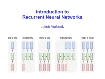
Variants on recurrent nets Images from Karpathy • 1: Conventional MLP • 2: Sequence generation , e.g. image to caption • 3: Sequence based prediction or classification, e.g. Speech recognition, text classification 67

Variants Images from Karpathy • 1: Delayed sequence to sequence, e.g. machine translation • 2: Sequence to sequence, e.g. stock problem, label prediction • Etc… 68

Story so far • Time series analysis must consider past inputs along with current input • Looking into the infinite past requires recursion • NARX networks achieve this by feeding back the output to the input • “Simple” recurrent networks maintain separate “memory” or “context” units to retain some information about the past – But during learning the current error does not influence the past • State-space models retain information about the past through recurrent hidden states – These are “fully recurrent” networks – The initial values of the hidden states are generally learnable parameters as well • State-space models enable current error to update parameters in the past 69

How do we train the network Y(0) Y(1) Y(2) Y(T-2) Y(T-1) Y(T) h -1 X(0) X(1) X(2) X(T-2) X(T-1) X(T) t • Back propagation through time (BPTT) • Given a collection of sequence inputs – (𝐘 � , 𝐄 � ) , where – 𝐘 � = 𝑌 �,� , … , 𝑌 �,� – 𝐄 � = 𝐸 �,� , … , 𝐸 �,� • Train network parameters to minimize the error between the output of the network � �,� and the desired outputs �,� – This is the most generic setting. In other settings we just “remove” some of the input or output entries 70

Training: Forward pass Y(0) Y(1) Y(2) Y(T-2) Y(T-1) Y(T) h -1 X(0) X(1) X(2) X(T-2) X(T-1) X(T) t • For each training input: • Forward pass: pass the entire data sequence through the network, generate outputs 71

Recurrent Neural Net Assuming time-synchronous output # Assuming h(-1,*) is known # Assuming L hidden-state layers and an output layer # W c (*) and W r (*) are matrics, b(*) are vectors # W c are weights for inputs from current time # W r is recurrent weight applied to the previous time # W o are output layre weights for t = 0:T-1 # Including both ends of the index h(t,0) = x(t) # Vectors. Initialize h(0) to input for l = 1:L # hidden layers operate at time t z(t,l) = W c (l)h(t,l-1) + W r (l)h(t-1,l) + b(l) h(t,l) = tanh(z(t,l)) # Assuming tanh activ. z o (t) = W o h(t,L) + b o Subscript “c” – current Y(t) = softmax( z o (t) ) Subscript “r” – recurrent 72

Training: Computing gradients Y(0) Y(1) Y(2) Y(T-2) Y(T-1) Y(T) h -1 X(0) X(1) X(2) X(T-2) X(T-1) X(T) t • For each training input: • Backward pass: Compute gradients via backpropagation – Back Propagation Through Time 73

Back Propagation Through Time 𝑍(0) 𝑍(1) 𝑍(2) 𝑍(𝑈 − 2) 𝑍(𝑈 − 1) 𝑍(𝑈) h -1 𝑌(0) 𝑌(1) 𝑌(2) 𝑌(𝑈 − 2) 𝑌(𝑈 − 1) 𝑌(𝑈) Will only focus on one training instance All subscripts represent components and not training instance index 74

Back Propagation Through Time 𝐸𝐽𝑊 𝐸(1. . 𝑈) 𝑍(0) 𝑍(1) 𝑍(2) 𝑍(𝑈 − 2) 𝑍(𝑈 − 1) 𝑍(𝑈) h -1 𝑌(0) 𝑌(1) 𝑌(2) 𝑌(𝑈 − 2) 𝑌(𝑈 − 1) 𝑌(𝑈) • The divergence computed is between the sequence of outputs by the network and the desired sequence of outputs • DIV is a scalar function of a series of vectors! • This is not just the sum of the divergences at individual times  Unless we explicitly define it that way 75

Notation 𝐸𝐽𝑊 𝐸(1. . 𝑈) 𝑍(0) 𝑍(1) 𝑍(2) 𝑍(𝑈 − 2) 𝑍(𝑈 − 1) 𝑍(𝑈) � h -1 � 𝑌(0) 𝑌(1) 𝑌(2) 𝑌(𝑈 − 2) 𝑌(𝑈 − 1) 𝑌(𝑈) • ( ) is the output at time – is the ith output � � • is the pre-activation value of the neurons at the output layer at time t • is the output of the hidden layer at time – Assuming only one hidden layer in this example � • is the pre-activation value of the hidden layer at time 76

Back Propagation Through Time 𝐸𝐽𝑊 𝐸(1. . 𝑈) 𝑍(0) 𝑍(1) 𝑍(2) 𝑍(𝑈 − 2) 𝑍(𝑈 − 1) 𝑍(𝑈) h -1 𝑌(0) 𝑌(1) 𝑌(2) 𝑌(𝑈 − 2) 𝑌(𝑈 − 1) 𝑌(𝑈) First step of backprop: Compute ���� �� � (�) Note: DIV is a function of all outputs Y(0) … Y(T) In general we will be required to compute ���� as we will see. This can �� � (�) be a source of significant difficulty in many scenarios. 77

𝐸𝐽𝑊 𝐸𝑗𝑤(0) 𝐸𝑗𝑤(1) 𝐸𝑗𝑤(2) 𝐸𝑗𝑤(𝑈 − 2) 𝐸𝑗𝑤(𝑈 − 1) 𝐸𝑗𝑤(𝑈) 𝐸(𝑈) 𝑍(0) 𝑍(1) 𝑍(2) 𝑍(𝑈 − 2) 𝑍(𝑈 − 1) 𝑍(𝑈) h -1 𝑌(0) 𝑌(1) 𝑌(2) 𝑌(𝑈 − 2) 𝑌(𝑈 − 1) 𝑌(𝑈) Special case, when the overall divergence is a simple sum of local divergences at each time: Must compute Will usually get � � � 78

Back Propagation Through Time 𝐸𝐽𝑊 𝐸(1. . 𝑈) 𝑍(0) 𝑍(1) 𝑍(2) 𝑍(𝑈 − 2) 𝑍(𝑈 − 1) 𝑍(𝑈) h -1 𝑌(0) 𝑌(1) 𝑌(2) 𝑌(𝑈 − 2) 𝑌(𝑈 − 1) 𝑌(𝑈) First step of backprop: Compute ���� �� � (�) � (�) (�) � (�) (�) �(�) Vector output activation � � OR (�) (�) (�) (�) � � � � � � � 79

Back Propagation Through Time 𝐸𝐽𝑊 𝐸(1. . 𝑈) 𝑍(0) 𝑍(1) 𝑍(2) 𝑍(𝑈 − 2) 𝑍(𝑈 − 1) 𝑍(𝑈) h -1 𝑌(0) 𝑌(1) 𝑌(2) 𝑌(𝑈 − 2) 𝑌(𝑈 − 1) 𝑌(𝑈) (�) � (�) �� (�) (�) � � � � � � � � (�) � (�) (�) �(�) (�) (�) � � � 80

Back Propagation Through Time 𝐸𝐽𝑊 𝐸(1. . 𝑈) 𝑍(0) 𝑍(1) 𝑍(2) 𝑍(𝑈 − 2) 𝑍(𝑈 − 1) 𝑍(𝑈) h -1 𝑌(0) 𝑌(1) 𝑌(2) 𝑌(𝑈 − 2) 𝑌(𝑈 − 1) 𝑌(𝑈) � (�) �� (�) (�) (�) � � � � � � � (�) � � (�) � (�) (�) �� � 81

Back Propagation Through Time 𝐸𝐽𝑊 𝐸(1. . 𝑈) 𝑍(0) 𝑍(1) 𝑍(2) 𝑍(𝑈 − 2) 𝑍(𝑈 − 1) 𝑍(𝑈) h -1 𝑌(0) 𝑌(1) 𝑌(2) 𝑌(𝑈 − 2) 𝑌(𝑈 − 1) 𝑌(𝑈) � (�) (�) � (�) (�) � (�) (�) �(�) � � � � (�) � �� (�) (�) � (�) (�) � � �� � � � � � 82

Back Propagation Through Time 𝐸𝐽𝑊 𝐸(1. . 𝑈) 𝑍(0) 𝑍(1) 𝑍(2) 𝑍(𝑈 − 2) 𝑍(𝑈 − 1) 𝑍(𝑈) h -1 𝑌(0) 𝑌(1) 𝑌(2) 𝑌(𝑈 − 2) 𝑌(𝑈 − 1) 𝑌(𝑈) � (�) � � �� � (�) � (�) (�) 83

Back Propagation Through Time 𝐸𝐽𝑊 𝐸(1. . 𝑈) 𝑍(0) 𝑍(1) 𝑍(2) 𝑍(𝑈 − 2) 𝑍(𝑈 − 1) 𝑍(𝑈) h -1 𝑌(0) 𝑌(1) 𝑌(2) 𝑌(𝑈 − 2) 𝑌(𝑈 − 1) 𝑌(𝑈) � (��) � (�) (�) � � (�) � (��) � �� � �� � 84

Back Propagation Through Time 𝐸𝐽𝑊 𝐸(1. . 𝑈) 𝑍(0) 𝑍(1) 𝑍(2) 𝑍(𝑈 − 2) 𝑍(𝑈 − 1) 𝑍(𝑈) h -1 𝑌(0) 𝑌(1) 𝑌(2) 𝑌(𝑈 − 2) 𝑌(𝑈 − 1) 𝑌(𝑈) � (�) � � (�) (���) �(���) Vector output activation � � OR � � � � � � � � � � � 85

Back Propagation Through Time 𝐸𝐽𝑊 𝐸(1. . 𝑈) 𝑍(0) 𝑍(1) 𝑍(2) 𝑍(𝑈 − 2) 𝑍(𝑈 − 1) 𝑍(𝑈) h -1 𝑌(0) 𝑌(1) 𝑌(2) 𝑌(𝑈 − 2) 𝑌(𝑈 − 1) 𝑌(𝑈) (�) (��) �� �� � � � � � � � (�) (��) � � (���) � (�) (�) �(���) 86

Back Propagation Through Time 𝐸𝐽𝑊 𝐸(1. . 𝑈) 𝑍(0) 𝑍(1) 𝑍(2) 𝑍(𝑈 − 2) 𝑍(𝑈 − 1) 𝑍(𝑈) h -1 𝑌(0) 𝑌(1) 𝑌(2) 𝑌(𝑈 − 2) 𝑌(𝑈 − 1) 𝑌(𝑈) (�) (��) �� �� � � � � � � � � (�) � Note the addition �� � 87 � � (���) � (�)

Back Propagation Through Time 𝐸𝐽𝑊 𝐸(1. . 𝑈) 𝑍(0) 𝑍(1) 𝑍(2) 𝑍(𝑈 − 2) 𝑍(𝑈 − 1) 𝑍(𝑈) h -1 𝑌(0) 𝑌(1) 𝑌(2) 𝑌(𝑈 − 2) 𝑌(𝑈 − 1) 𝑌(𝑈) � � � � � � � � ��� � (�) (���) �(���) 88

Back Propagation Through Time 𝐸𝐽𝑊 𝐸(1. . 𝑈) 𝑍(0) 𝑍(1) 𝑍(2) 𝑍(𝑈 − 2) 𝑍(𝑈 − 1) 𝑍(𝑈) h -1 𝑌(0) 𝑌(1) 𝑌(2) 𝑌(𝑈 − 2) 𝑌(𝑈 − 1) 𝑌(𝑈) � � (�) � � � �� � � � � Note the addition � � (���) � (�) 89

Back Propagation Through Time 𝐸𝐽𝑊 𝐸(1. . 𝑈) 𝑍(0) 𝑍(1) 𝑍(2) 𝑍(𝑈 − 2) 𝑍(𝑈 − 1) 𝑍(𝑈) h -1 𝑌(0) 𝑌(1) 𝑌(2) 𝑌(𝑈 − 2) 𝑌(𝑈 − 1) 𝑌(𝑈) � (�) � �� � � Note the addition (��) � � �� 90 � � (���) � (��)

Back Propagation Through Time 𝐸𝐽𝑊 𝐸(1. . 𝑈) 𝑍(0) 𝑍(1) 𝑍(2) 𝑍(𝑈 − 2) 𝑍(𝑈 − 1) 𝑍(𝑈) h -1 𝑌(0) 𝑌(1) 𝑌(2) 𝑌(𝑈 − 2) 𝑌(𝑈 − 1) 𝑌(𝑈) Continue computing derivatives (��) going backward through time until.. �� � 𝑗 � � (��) � � (�) � �� 91

Back Propagation Through Time 𝐸𝐽𝑊 𝐸(1. . 𝑈) 𝑍(0) 𝑍(1) 𝑍(2) 𝑍(𝑈 − 2) 𝑍(𝑈 − 1) 𝑍(𝑈) h -1 𝑌(0) 𝑌(1) 𝑌(2) 𝑌(𝑈 − 2) 𝑌(𝑈 − 1) 𝑌(𝑈) (���) (�,�) �,� �,� � ��� � � � � � � Not showing derivatives � � at output neurons � � � � 92 � �

Back Propagation Through Time 𝐸𝐽𝑊 𝐸(1. . 𝑈) 𝑍(0) 𝑍(1) 𝑍(2) 𝑍(𝑈 − 2) 𝑍(𝑈 − 1) 𝑍(𝑈) h -1 𝑌(0) 𝑌(1) 𝑌(2) 𝑌(𝑈 − 2) 𝑌(𝑈 − 1) 𝑌(𝑈) (��) �� � 𝑗 � � � � (�) � (��) � �� � � � � �� 93

BPTT # Assuming forward pass has been completed # Jacobian(x,y) is the jacobian of x w.r.t. y # Assuming dY(t) = gradient(div,Y(t)) available for all t # Assuming all dz, dh, dW and db are initialized to 0 for t = T-1:downto:0 # Backward through time dz o (t) = dY(t)Jacobian(Y(t),z o (t)) dW o += h(t,L)dz o (t) db o += dz o (t) dh(t,L) += dz o (t)W o for l = L:1 # Reverse through layers dz(t,l) = dh(t,l)Jacobian(h(t,l),z(t,l)) dh(t,l-1) += dz(t,l) W c (l) dh(t-1,l) = dz(t,l) W r (l) Subscript “c” – current Subscript “r” – recurrent dW c (l) += h(t,l-1)dz(t,l) dW r (l) += h(t-1,l)dz(t,l) db(l) += dz(t,l) 94

BPTT • Can be generalized to any architecture 95

Extensions to the RNN: Bidirectional RNN Proposed by Schuster and Paliwal 1997 • RNN with both forward and backward recursion – Explicitly models the fact that just as the future can be predicted from the past, the past can be deduced from the future 96

Bidirectional RNN Y(0) Y(1) Y(2) Y(T-2) Y(T-1) Y(T) h f (-1) X(0) X(1) X(2) X(T-2) X(T-1) X(T) h b (inf) X(0) X(1) X(2) X(T-2) X(T-1) X(T) t • A forward net process the data from t=0 to t=T • A backward net processes it backward from t=T down to t=0 97

Bidirectional RNN: Processing an input string h f (-1) X(0) X(1) X(2) X(T-2) X(T-1) X(T) t • The forward net process the data from t=0 to t=T – Only computing the hidden states, initially • The backward net processes it backward from t=T down to t=0 98

Bidirectional RNN: Processing an input string h f (-1) X(0) X(1) X(2) X(T-2) X(T-1) X(T) h b (inf) X(0) X(1) X(2) X(T-2) X(T-1) X(T) t • The backward nets processes the input data in reverse time, end to beginning – Initially only the hidden state values are computed • Clearly, this is not an online process and requires the entire input data – Note: This is not the backward pass of backprop. net processes it backward from t=T down to t=0 99

Bidirectional RNN: Processing an input string Y(0) Y(1) Y(2) Y(T-2) Y(T-1) Y(T) h f (-1) X(0) X(1) X(2) X(T-2) X(T-1) X(T) h b (inf) X(0) X(1) X(2) X(T-2) X(T-1) X(T) t • The computed states of both networks are used to compute the final output at each time 100