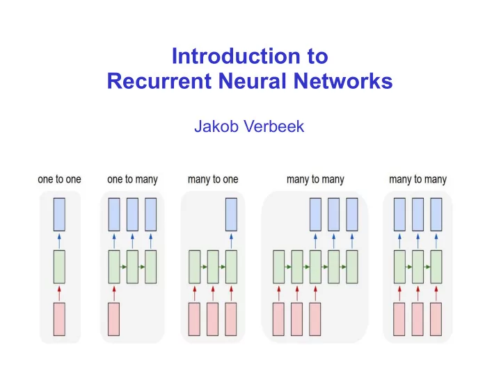
Introduction to Recurrent Neural Networks Jakob Verbeek Modeling - PowerPoint PPT Presentation

Introduction to Recurrent Neural Networks Jakob Verbeek

Modeling sequential data with Recurrent Neural Networks Compact schematic drawing of standard multi-layer perceptron (MLP)  output hidden input

Modeling sequential data So far we considered “one-to-one” prediction tasks  Classification: one image to one class label, which digit is displayed 0...9 ► Regression: one image to one scalar, how old is this person? ► Many prediction problems have a sequential nature to them  Either in input, in output, or both ► Both may vary in length from one example to another ►

Modeling sequential data One-to-many prediction  Image captioning  Input: an image ► Output: natural language description, ► variable length sequence of words

Modeling sequential data Text classification  Input: a sentence ► Output: user rating ►

Modeling sequential data Machine translation of text from one language to another  Sequences of different length on input and output ►

Modeling sequential data Part of speech tagging  For each word in sentence predict PoS label (verb, noun, adjective, etc.) ► Temporal segmentation of video  Predict action label for every video frame ► Temporal segmentation of audio  Predict phoneme labels over time ►

Modeling sequential data Possible to use a k-order autoregressive model over output sequences  Limits memory to only k time steps in the past ► Not applicable when input sequence is not aligned with output sequence  Many-to-one tasks, unaligned many-to-many ►

Recurrent neural networks Recurrent computation of hidden units from one time step to the next  Hidden state accumulates information on entire sequence, since the field ► of view spans entire sequence processed so far Time-invariant function makes it applicable to arbitrarily long sequences ► Similar ideas used in  Hidden Markov models for arbitrarily long sequences ► Parameter sharing across space in convolutional neural networks ► But has limited field of view: parallel instead of sequential processing 

Recurrent neural networks Basic example for many-to-many prediction  Hidden state linear function of current input and previous hidden state, ► followed by point-wise non-linearity Output is linear function of current hidden state, followed by point-wise ► non-linearity z t =ϕ( A x t + B z t − 1 ) y t =ψ( C z t ) y t z t x t

Recurrent neural network diagrams Two graphical representations are used  “Unfolded” flow diagram Recurrent flow diagram y t y t C z t =ϕ ( A x t + B z t − 1 ) B z t z t y t =ψ( C z t ) A x t x t Unfolded representation shows that we still have an acyclic directed graph  Size of the graph (horizontally) is variable, given by sequence length ► Weights are shared across horizontal replications ► Gradient computation via back-propagation as before  Referred to as “back-propagation through time” (Pearlmutter, 1989) ►

Recurrent neural network diagrams Deterministic feed-forward network from inputs to outputs  Predictive model over output sequence is obtained by defining a distribution  over outputs given y For example: probability of a word given via softmax of word score ► Training loss: sum of losses over output variables  Independent prediction of elements in output given input sequence ► T L =− ∑ t = 1 ln p ( w t ∣ x 1: t ) w t y t z t =ϕ( A x t + B z t − 1 ) y t =ψ( C z t ) z t exp y tk p ( w t = k ∣ x 1: t )= V ∑ v = 1 exp y tv x t

More topologies: “deep” recurrent networks Instead of a recurrence across a single hidden layer, consider a recurrence  across a multi-layer architecture t t t t y y y y t t t t h h h h t t z t t z z z t t t t x x x x

More topologies: multi-dimensional recurrent networks Instead of a recurrence across a single (time) axis, consider a recurrence  across a multi-dimensional grid For example: axis aligned directed edges  Each node receives input from predecessors, one for each dimension ► 3,1 3,2 3,3 x x x 3,1 3,2 3,3 x x x 2,1 2,2 2,3 x x x 2,1 2,2 2,3 x x x 1,1 1,2 1,3 x x x 1,1 1,2 1,3 x x x

More topologies: bidirectional recurrent neural networks Standard RNN only uses left-context for many-to-many prediction  Use two separate recurrences, one in each direction  Aggregate output from both directions for prediction at each time step ► Only possible on a given input sequence of arbitrary length  Not on output sequence, since it needs to be predicted/generated ►

More topologies: output feedback loops So far the element in the output sequence at time t was independently drawn  given the state at time t State at time t depends on the entire input sequence up to time t ► No dependence on the output sequence produced so far ► Problematic when there are strong regularities in output, eg character or  words sequences in natural language T p ( w 1: T ∣ x 1: T )= ∏ t = 1 p ( w t ∣ x 1: t ) y t z t x t

More topologies: output feedback loops To introduce dependence on output sequence, we add a feedback loop from  the output to the hidden state T p ( y 1: T ∣ x 1: T )= ∏ t = 1 p ( y t ∣ x 1: t , y 1: t − 1 ) y t z t x t Without output-feedback, the state evolution is a deterministic non-linear  dynamical system With output feedback, the state evolution becomes a stochastic non-linear  dynamical system Caused by the stochastic output, which flows back into the state update ►

How do we generate data from an RNN ? RNN gives a distribution over output sequences  Sampling: sequentially sample one element at a time  Compute state from current input and previous state and output ► Compute distribution on current output symbol ► Sample output symbol ► Compute maximum likelihood sequence?  Not feasible with feedback since output symbol impacts state ► y t Marginal distribution on n-th symbol  Not feasible: marginalize over exponential nr. of sequences ► z t Marginal probability of a symbol appearing anywhere in seq.  Not feasible: average over all marginals ► x t

Approximate maximum likelihood sequences Exhaustive maximum likelihood search exponential in sequence length  Use Beam Search, computational cost linear in  Beam size K, vocabulary size V, (maximum) sequence length T ► T = 1 T = 2 T = 3 current proposed current proposed current proposed extensions extensions extensions hypotheses hypotheses hypotheses ϵ ϵ ϵ ϵ a ϵ a a λ a b b b ϵ ϵ empty a a a ϵ a string b b ϵ ϵ a a a b b b b

Ensembles of networks to improve prediction Averaging predictions of several networks can improve results  Trained from different initialization and using different mini-batches ► Possibly including networks with different architectures, but not per se ► For CNNs see eg [Krizhevsky & Hinton, 2012] [Simomyan & Zisserman, 2014] ► For RNN sequence prediction  Train RNNs independently ► “Run” RNNs in parallel for prediction, updating states with common seq. ► Average distribution over next symbol ► Sample or beam-search based on av. distribution ► A B ? A B ?

How to train an RNN without output feedback? Compute full state sequence given the input (deterministic given input)  Compute loss at each time step w.r.t. ground truth output sequence  Backpropagation (“through time”) to compute gradients w.r.t. loss  y t z t x t

How to train an RNN with output feedback? Compute state sequence given input and ground-truth output,  deterministic due to known and fixed output Loss at each time step wrt ground truth output seq, backprop through time  Note discrepancy between train and test  Train: predict next symbol from ground-truth sequence so far ► Test: predict next symbol from generated sequence so far ► Might deviate from observed ground-truth sequences  y t z t x t

Scheduled sampling for RNN training Compensate discrepancy between train and test procedure by training from  generated sequence [Bengio et al. NIPS, 2015] Learn to recover from partially incorrect sequences ► Directly training from sampled sequences does not work well in practice  At the start randomly initialized model generates random sequences ► Instead, start by training from ground-truth sequence, and progressively ► increase probability to sample generated symbol in the sequence

Scheduled sampling for RNN training Evaluation image captioning  Image in, sentence out ► Higher scores are better ► Scheduled sampling improves baseline, also in ensemble case  Uniform Scheduled Sampling: sample uniform instead of using model  Already improves over baseline, but not as much as using model ► Always sampling gives very poor results, as expected 