Differential Categories, Recurrent Neural Networks, and Machine - PowerPoint PPT Presentation
Differential Categories, Recurrent Neural Networks, and Machine Learning Shin-ya Katsumata and David Sprunger* National Institute of Informatics, Tokyo SYCO 4 Chapman University May 23, 2019 1/32 Outline Feedforward neural networks 1
Differential Categories, Recurrent Neural Networks, and Machine Learning Shin-ya Katsumata and David Sprunger* National Institute of Informatics, Tokyo SYCO 4 Chapman University May 23, 2019 1/32
Outline Feedforward neural networks 1 Recurrent neural networks 2 Cartesian differential categories 3 Stateful computations / functions 4 Lifting Cartesian differential structure to stateful functions 5 2/32
Overview of neural networks A neural network is a function with two types of arguments, data inputs and parameters . Data come from the environment, parameters are controlled by us. As a string diagram: parameters: θ ∈ R k output: y ∈ R m φ data inputs: x ∈ R n 3/32
Overview of neural networks A neural network is a function with two types of arguments, data inputs and parameters . Data come from the environment, parameters are controlled by us. As a string diagram: parameters: θ ∈ R k output: y ∈ R m φ data inputs: x ∈ R n Training a neural network means finding θ ∗ : 1 → R k so that θ ∗ φ has a desired property. 3/32
Overview of neural networks A neural network is a function with two types of arguments, data inputs and parameters . Data come from the environment, parameters are controlled by us. As a string diagram: parameters: θ ∈ R k output: y ∈ R m φ data inputs: x ∈ R n Training a neural network means finding θ ∗ : 1 → R k so that θ ∗ φ has a desired property. Usually, this means minimizing inaccuracy, as measured by θ ∗ φ ˆ E R x i ˆ y i y i � : 1 → R n + m are given input-output pairs and where � ˆ x i , ˆ E : R m × R m → R is a given error function. 3/32
Overview of neural networks Gradient-based training algorithms utilize the insight that the gradient of this function: R k φ ˆ E R x i ˆ y i tells us how to modify θ in order to decrease the error quickest. 4/32
Overview of neural networks Gradient-based training algorithms utilize the insight that the gradient of this function: R k φ ˆ E R x i ˆ y i tells us how to modify θ in order to decrease the error quickest. Backpropagation is an algorithm that finds gradients (or derivatives) of functions f : R n → R m , and is often used due to its performance when n ≫ m . 4/32
Overview of neural networks Gradient-based training algorithms utilize the insight that the gradient of this function: R k φ ˆ E R x i ˆ y i tells us how to modify θ in order to decrease the error quickest. Backpropagation is an algorithm that finds gradients (or derivatives) of functions f : R n → R m , and is often used due to its performance when n ≫ m . Backprop generates a hint about which direction to change θ , but the trainer determines how this hint is used. 4/32
Outline Feedforward neural networks 1 Recurrent neural networks 2 Cartesian differential categories 3 Stateful computations / functions 4 Lifting Cartesian differential structure to stateful functions 5 5/32
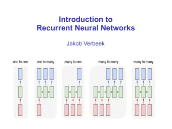
Recurrent neural networks Recurrent neural networks (RNNs) are able to process variable-length inputs using state , which is stored in registers : i Ψ : ψ x y 6/32
Recurrent neural networks Recurrent neural networks (RNNs) are able to process variable-length inputs using state , which is stored in registers : i Ψ : ψ x y A common semantics of RNNs uses the unrollings of the network: i ψ U 0 Ψ : y 0 x 0 i ψ U 1 Ψ : x 0 ψ y 1 x 1 i ψ U 2 Ψ : x 0 ψ x 1 ψ y 2 x 2 6/32
Backpropagation through time Infinite-dimensional derivatives for sequence-to-sequence functions must be approximated to be computationally useful. 7/32
Backpropagation through time Infinite-dimensional derivatives for sequence-to-sequence functions must be approximated to be computationally useful. Backpropagation through time (BPTT) : Whenever the derivative of Ψ is needed at an input of length k + 1 , the derivative of U k Ψ is used instead. 7/32
Backpropagation through time Infinite-dimensional derivatives for sequence-to-sequence functions must be approximated to be computationally useful. Backpropagation through time (BPTT) : Whenever the derivative of Ψ is needed at an input of length k + 1 , the derivative of U k Ψ is used instead. This is a good way to generate hints, but it opens some questions: 1 U k ( Ψ ◦ Φ ) � = U k Ψ ◦ U k Φ . Did we lose the chain rule? What properties of derivatives hold for BPTT? 7/32
Backpropagation through time Infinite-dimensional derivatives for sequence-to-sequence functions must be approximated to be computationally useful. Backpropagation through time (BPTT) : Whenever the derivative of Ψ is needed at an input of length k + 1 , the derivative of U k Ψ is used instead. This is a good way to generate hints, but it opens some questions: 1 U k ( Ψ ◦ Φ ) � = U k Ψ ◦ U k Φ . Did we lose the chain rule? What properties of derivatives hold for BPTT? 2 U k Ψ and U k +1 Ψ have a lot in common, so their derivatives should as well. Is there a more compact representation for the derivative of Ψ than a sequence of functions? 7/32
Understanding BPTT with category theory The project: start in a category with some notion of derivative, add a mechanism for state, and extend the original notion of differentiation to the stateful setting. Two main parts: 1 Adding state to computations 2 Differentiation for stateful computations 8/32
Understanding BPTT with category theory The project: start in a category with some notion of derivative, add a mechanism for state, and extend the original notion of differentiation to the stateful setting. Two main parts: 1 Adding state to computations Relatively common, back to Katis, Sabadini, & Walters ‘97 1 Digital circuits—Ghica & Jung, ‘16 2 Signal flow graphs—Bonchi, Soboci´ nski, & Zanasi, ‘14 3 2 Differentiation for stateful computations 8/32
Understanding BPTT with category theory The project: start in a category with some notion of derivative, add a mechanism for state, and extend the original notion of differentiation to the stateful setting. Two main parts: 1 Adding state to computations Relatively common, back to Katis, Sabadini, & Walters ‘97 1 Digital circuits—Ghica & Jung, ‘16 2 Signal flow graphs—Bonchi, Soboci´ nski, & Zanasi, ‘14 3 2 Differentiation for stateful computations Not so common 1 Cartesian differential categories—Blute, Cockett, Seely ‘09 2 (Backprop as Functor—Fong, Spivak, Tuy´ eras, ‘17) 3 (Simple Essence of Automatic Differentiation—Elliott ‘18) 4 8/32
Outline Feedforward neural networks 1 Recurrent neural networks 2 Cartesian differential categories 3 Stateful computations / functions 4 Lifting Cartesian differential structure to stateful functions 5 9/32
Cartesian differential categories [Blute, Cockett, Seely ’09] A Cartesian differential category has a differential operation on morphisms sending f : X → Y to Df : X × X → Y , satisfying seven axioms: s Ds = for s ∈ { id X , σ X,Y , ! X , ∆ X , 0 X , + X } . CD1. 0 0 Df = CD2. Df + + Df = CD3. Df Df CD4. D ( ) g Dg = f f g Dg D ( ) = CD5. f Df 10/32
Cartesian differential category axioms, continued = CD6. 0 DDf Df = CD7. DDf DDf 11/32
Cartesian differential category axioms, continued = CD6. 0 DDf Df = CD7. DDf DDf Example Objects of the category Euc ∞ are R n for n ∈ N , maps are smooth maps between them. Euc ∞ is a Cartesian differential category with the (curried) Jacobian sending f : R n → R m to Df : (∆ x, x ) �→ Jf | x × ∆ x . 11/32
Differentiating the unrollings of a simple RNN 0 i D ( ) ψ Dψ = i 12/32
Differentiating the unrollings of a simple RNN 0 i D ( ) ψ Dψ = i 0 Dψ i ψ D ( ) = ψ i Dψ ψ 12/32
Differentiating the unrollings of a simple RNN 0 i D ( ) ψ Dψ = i 0 Dψ i ψ D ( ) = ψ i Dψ ψ 0 i Dψ ψ D ( ) ψ = ψ i Dψ ψ Dψ ψ 12/32
0 i Dψ ψ D ( ) ψ = ψ i Dψ ψ Dψ ψ This suggests a hypothesis: 13/32
0 i Dψ ψ D ( ) ψ = ψ i Dψ ψ Dψ ψ This suggests a hypothesis: 0 D ∗ ψ D ∗ i � ψ i ψ 13/32
Outline Feedforward neural networks 1 Recurrent neural networks 2 Cartesian differential categories 3 Stateful computations / functions 4 Lifting Cartesian differential structure to stateful functions 5 14/32
Stateful computations Let ( C , × , 1) be a strict Cartesian category, whose morphisms we 1 think of as stateless functions. A 1 i ·· 1 stateful sequence computation looks like this: S 0 X 0 Ψ 0 Y 0 S 1 X 1 Ψ 1 Y 1 S 2 . . . 15/32
Stateful computations Let ( C , × , 1) be a strict Cartesian category, whose morphisms we 1 think of as stateless functions. A 1 ·· i 1 stateful sequence computation looks like this: S 0 X 0 Ψ 0 Y 0 (This is a sequence of 2-cells in a double category based on C , with S 1 a restriction on the first 2-cell.) X 1 Ψ 1 Y 1 S 2 . . . 15/32
Stateful functions Two computation sequences might have different state spaces and still compute the same function. For example: 1 1 1 1 1 ·· i 1 1 S X 0 X 0 X 0 X 0 1 S X 1 X 1 X 1 X 1 1 S . . . . . . 16/32
Recommend
More recommend
Explore More Topics
Stay informed with curated content and fresh updates.
