Recognition Topics that we will try to cover: Indexing for fast - PowerPoint PPT Presentation
Recognition Topics that we will try to cover: Indexing for fast retrieval (we still owe this one) Object classification (we did this one already) Neural Networks Object class detection Hough-voting techniques Support Vector Machines (SVM)
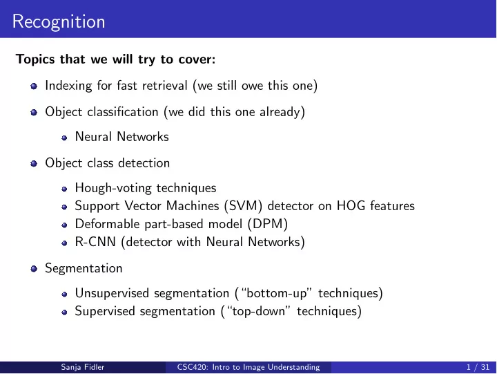
Recognition Topics that we will try to cover: Indexing for fast retrieval (we still owe this one) Object classification (we did this one already) Neural Networks Object class detection Hough-voting techniques Support Vector Machines (SVM) detector on HOG features Deformable part-based model (DPM) R-CNN (detector with Neural Networks) Segmentation Unsupervised segmentation (“bottom-up” techniques) Supervised segmentation (“top-down” techniques) Sanja Fidler CSC420: Intro to Image Understanding 1 / 31
Recognition: Indexing for Fast Retrieval Sanja Fidler CSC420: Intro to Image Understanding 2 / 31
Recognizing or Retrieving Specific Objects Example: Visual search in feature films Demo: http://www.robots.ox.ac.uk/~vgg/research/vgoogle/ [Source: J. Sivic, slide credit: R. Urtasun] Sanja Fidler CSC420: Intro to Image Understanding 3 / 31
Recognizing or Retrieving Specific Objects Example: Search photos on the web for particular places [Source: J. Sivic, slide credit: R. Urtasun] Sanja Fidler CSC420: Intro to Image Understanding 4 / 31
Sanja Fidler CSC420: Intro to Image Understanding 5 / 31
Why is it Di ffi cult? Objects can have possibly large changes in scale, viewpoint, lighting and partial occlusion. [Source: J. Sivic, slide credit: R. Urtasun] Sanja Fidler CSC420: Intro to Image Understanding 6 / 31
Why is it Di ffi cult? There is tones of data. Sanja Fidler CSC420: Intro to Image Understanding 7 / 31
Our Case: Matching with Local Features For each image in our database we extracted local descriptors (e.g., SIFT) Sanja Fidler CSC420: Intro to Image Understanding 8 / 31
Our Case: Matching with Local Features For each image in our database we extracted local descriptors (e.g., SIFT) Sanja Fidler CSC420: Intro to Image Understanding 8 / 31
Our Case: Matching with Local Features Let’s focus on descriptors only (vectors of e.g. 128 dim for SIFT) Sanja Fidler CSC420: Intro to Image Understanding 8 / 31
Our Case: Matching with Local Features Sanja Fidler CSC420: Intro to Image Understanding 8 / 31
Our Case: Matching with Local Features Sanja Fidler CSC420: Intro to Image Understanding 8 / 31
Our Case: Matching with Local Features Sanja Fidler CSC420: Intro to Image Understanding 8 / 31
Indexing! Sanja Fidler CSC420: Intro to Image Understanding 9 / 31
Indexing Local Features: Inverted File Index For text documents, an e ffi cient way to find all pages on which a word occurs is to use an index. We want to find all images in which a feature occurs. To use this idea, well need to map our features to “visual words”. Why? [Source: K. Grauman, slide credit: R. Urtasun] Sanja Fidler CSC420: Intro to Image Understanding 10 / 31
How would “visual words” help us? Sanja Fidler CSC420: Intro to Image Understanding 11 / 31
How would “visual words” help us? Sanja Fidler CSC420: Intro to Image Understanding 11 / 31
How would “visual words” help us? Sanja Fidler CSC420: Intro to Image Understanding 11 / 31
How would “visual words” help us? Sanja Fidler CSC420: Intro to Image Understanding 11 / 31
But What Are Our Visual “Words”? Sanja Fidler CSC420: Intro to Image Understanding 12 / 31
But What Are Our Visual “Words”? Sanja Fidler CSC420: Intro to Image Understanding 12 / 31
But What Are Our Visual “Words”? Sanja Fidler CSC420: Intro to Image Understanding 12 / 31
But What Are Our Visual “Words”? Sanja Fidler CSC420: Intro to Image Understanding 12 / 31
But What Are Our Visual “Words”? Sanja Fidler CSC420: Intro to Image Understanding 12 / 31
But What Are Our Visual “Words”? Sanja Fidler CSC420: Intro to Image Understanding 12 / 31
But What Are Our Visual “Words”? Sanja Fidler CSC420: Intro to Image Understanding 12 / 31
Visual Words All example patches on the right belong to the same visual word. [Source: R. Urtasun] Sanja Fidler CSC420: Intro to Image Understanding 13 / 31
Now We Can do Our Fast Matching Sanja Fidler CSC420: Intro to Image Understanding 14 / 31
Inverted File Index Now we found all images in the database that have at least one visual word in common with the query image But this can still give us lots of images... What can we do? Sanja Fidler CSC420: Intro to Image Understanding 15 / 31
Inverted File Index Now we found all images in the database that have at least one visual word in common with the query image But this can still give us lots of images... What can we do? Idea: Compute meaningful similarity (e ffi ciently) between query image and retrieved images. Then just match query to top K most similar images and forget about the rest. Sanja Fidler CSC420: Intro to Image Understanding 15 / 31
Inverted File Index Now we found all images in the database that have at least one visual word in common with the query image But this can still give us lots of images... What can we do? Idea: Compute meaningful similarity (e ffi ciently) between query image and retrieved images. Then just match query to top K most similar images and forget about the rest. How can we do compute a meaningful similarity, and do it fast? Sanja Fidler CSC420: Intro to Image Understanding 15 / 31
Relation to Documents [Slide credit: R. Urtasun] Sanja Fidler CSC420: Intro to Image Understanding 16 / 31
Bags of Visual Words [Slide credit: R. Urtasun] Summarize entire image based on its distribution (histogram) of word occurrences. Analogous to bag of words representation commonly used for documents. Sanja Fidler CSC420: Intro to Image Understanding 17 / 31
Compute a Bag-of-Words Description Sanja Fidler CSC420: Intro to Image Understanding 18 / 31
Compute a Bag-of-Words Description Sanja Fidler CSC420: Intro to Image Understanding 18 / 31
Compute a Bag-of-Words Description Sanja Fidler CSC420: Intro to Image Understanding 18 / 31
Comparing Images Compute the similarity by normalized dot product between their representations (vectors) sim( t j , q ) = < t j , q > || t j || · || q || Rank images in database based on the similarity score (the higher the better) Take top K best ranked images and do spatial verification (compute transformation and count inliers) Sanja Fidler CSC420: Intro to Image Understanding 19 / 31
Comparing Images Compute the similarity by normalized dot product between their representations (vectors) sim( t j , q ) = < t j , q > || t j || · || q || Rank images in database based on the similarity score (the higher the better) Take top K best ranked images and do spatial verification (compute transformation and count inliers) Sanja Fidler CSC420: Intro to Image Understanding 19 / 31
Compute a Better Bag-of-Words Description Sanja Fidler CSC420: Intro to Image Understanding 20 / 31
Compute a Better Bag-of-Words Description Sanja Fidler CSC420: Intro to Image Understanding 20 / 31
Compute a Better Bag-of-Words Description Instead of a histogram, for retrieval it’s better to re-weight the image description vector t = [ t 1 , t 2 , . . . , t i , . . . ] with term frequency-inverse document frequency (tf-idf), a standard trick in document retrieval: t i = n id log N n d n i where: is the number of occurrences of word i in image d n id . . . is the total number of words in image d n d . . . is the number of occurrences of word i in the whole database n i . . . is the number of documents in the whole database N . . . Sanja Fidler CSC420: Intro to Image Understanding 20 / 31
Compute a Better Bag-of-Words Description Instead of a histogram, for retrieval it’s better to re-weight the image description vector t = [ t 1 , t 2 , . . . , t i , . . . ] with term frequency-inverse document frequency (tf-idf), a standard trick in document retrieval: t i = n id log N n d n i where: is the number of occurrences of word i in image d n id . . . is the total number of words in image d n d . . . is the number of occurrences of word i in the whole database n i . . . is the number of documents in the whole database N . . . The weighting is a product of two terms: the word frequency n id n d , and the inverse document frequency log N n i Sanja Fidler CSC420: Intro to Image Understanding 20 / 31
Compute a Better Bag-of-Words Description Instead of a histogram, for retrieval it’s better to re-weight the image description vector t = [ t 1 , t 2 , . . . , t i , . . . ] with term frequency-inverse document frequency (tf-idf), a standard trick in document retrieval: t i = n id log N n d n i where: is the number of occurrences of word i in image d n id . . . is the total number of words in image d n d . . . is the number of occurrences of word i in the whole database n i . . . is the number of documents in the whole database N . . . The weighting is a product of two terms: the word frequency n id n d , and the inverse document frequency log N n i Intuition behind this: word frequency weights words occurring often in a particular document, and thus describe it well, while the inverse document frequency downweights the words that occur often in the full dataset Sanja Fidler CSC420: Intro to Image Understanding 20 / 31
Recommend
More recommend
Explore More Topics
Stay informed with curated content and fresh updates.
