HMMS and Speech HMMS and Speech HMMS and Speech Recognition - PowerPoint PPT Presentation
HMMS and Speech HMMS and Speech HMMS and Speech Recognition Recognition Recognition Presented by Jen-Wei Kuo Reference 1. X. Huang et. al., Spoken Language Processing, Chapter 8 2. Daniel Jurafsky and James H. Martin, Speech and Language
HMMS and Speech HMMS and Speech HMMS and Speech Recognition Recognition Recognition Presented by Jen-Wei Kuo
Reference 1. X. Huang et. al., Spoken Language Processing, Chapter 8 2. Daniel Jurafsky and James H. Martin, Speech and Language Processing, Chapter 7 3. Berlin Chen, Fall, 2002: Speech Signal Processing, Hidden Markov Models for Speech Recognition
Outline Overview of Speech Recognition Architecture Overview of Hidden Markov Models The Viterbi Algorithm Revisited Advanced Methods for Decoding A* Decoding Acoustic Processing of Speech Sound Waves How to Interpret a Waveform Spectra Feature Extraction
Outline (Cont.) Computing Acoustic Probabilities Training a Speech Recognizer Waveform Generation for Speech Synthesis Pitch and Duration Modification Unit Selection Human Speech Recognition Summary
HMMs and Speech Recognition Application : Large – Vocabulary Continuous Speech Recognition (LVCSR) Large vocabulary : Dictionary size 5000 – 60000 words Isolated – word speech : each word followed by a pause Continuous speech : words are run together naturally Speaker-independent
Speech Recognition Architecture ↓ Figure 5.1 The noisy channel model of individual words Acoustic input considered a noisy version of a source sentence. ↑ Figure 7.1 The noisy channel model applied to entire sentences
Speech Recognition Architecture Implementing the noisy-channel model have two problems. Metric for selecting best match? probability Efficient algorithm for finding best match? A* Modern Speech Recognizer Providing a search through a huge space of potential ”source” sentences. And choosing the one which has the highest probability of generating this sentence. So they use models to express the probability of words. N-grams and HMMs are applied.
Speech Recognition Architecture The goal of the probabilistic noisy channel architecture for speech recognition can be summarized as follows : What is the most likely sentence out of all sentences in the language L given some acoustic input O ?
Speech Recognition Architecture = Observations : O o , o , o , , o L 1 2 3 t = Word Sequences : W w , w , w , , w L 1 2 3 n Probabilistic implementation can be expressed : ˆ = W arg max P ( W | O ) W ∈ L Then we can use Bayes ’ rule to break it down : P ( O | W ) P ( W ) ˆ = = W arg max P ( W | O ) arg max P ( O ) ∈ ∈ W L W L P ( WO ) P ( WO ) = = P ( W | O ) and P ( O | W ) Q P ( O ) P ( W ) ∴ ⋅ = = ⋅ P ( W | O ) P ( O ) P ( WO ) P ( O | W ) P ( W )
Speech Recognition Architecture For each potential sentence we are still examining the same observations O , which must have the same probability P(O). ˆ = Posterior probability W arg max P ( W | O ) ∈ W L P ( O | W ) P ( W ) = = arg max arg max P ( O | W ) P ( W ) P ( O ) ∈ ∈ W L W L Observation likelihood Prior probability Acoustic model Language model
Speech Recognition Architecture Errata! page 239, line -7:Change “ can be computing ” to “ can be computed ” . Three stage for speech recognition system Signal processing or Feature extraction stage : Waveform is sliced up into frames. Waveform are transformed into spectral features. Subword or Phone recognition stage : Recognize individual speech. Decoding stage : Find the sequence of words that most probably generated the input. Errata! page 240, line -12:Delete extraneous closing paren. “ ) ( ”
Speech Recognition Architecture ↓ Figure 7.2 Schematic architecture for a speech recognition
Overview of HMMs Previously, Markov chains used to model pronounciation ↓ Figure 7.3 A simple weighted automaton or Markov chain pronunciation network for the work need. a The transition probabilities between two xy states x and y are 1.0 unless otherwise specified.
Overview of HMMs Forward algorithm:Phone sequences likelihood. Real input is not symbolic: Spectral features input symbols do not correspond to machine states HMM definition: State set Q. Observation symbols O ≠ Q. a a a a n a Transition probabilities A = 01 02 03 1 nn Observation likelihood B = b j o ( ) t Two special states:start state and end state π Initial distribution: is the probability that the i HMM will start in state i.
Overview of HMMs ↑ Figure 7.4 An HMM pronunciation network for the word need. Compared with Markov Chain : Separate set of observation symbols O. Likelihood function B is not limited to 0 or 1.
Overview of HMMs Visible ( Observable ) Markov Model One state , one event . States which the machine passed through is known. Too simple to describe the speech signal characteristics.
The Viterbi Algorithm Revisited Viterbi algorithm: Find the most-likely path through the automaton Word boundaries unknow in continuous speech If we know where the word boundaries. we can sure the pronunciation came from one word. Then, we only had some candidates to compare. But it’s the lack of spaces indicating word boundaries. It make the task difficult. Segmentation The task of finding word boundaries in connected speech. It will solve it by using the Viterbi algorithm.
The Viterbi Algorithm Revisited Errata! page 246, Figure 7.6: Change “ i ” to “ iy ” on x axis. iy ↑ Figure 7.6 Result of the Viterbi algorithm used to find the most-likely phone sequence
The Viterbi Algorithm Revisited = = λ viterbi [ t , j ] max P ( q q ... q q j , o o ... o | ) − 1 2 t 1 , t 1 2 t q , q ,..., q − 1 2 t 1 = − max ( viterbi [ t 1 , i ] a ) b ( o ) ij j t i Assumption of Viterbi algorithm: Dynamic programming invariant If ultimate best path for O includes state q i , that this best path must include the best path up to state q i This doesn’t mean that the best path at any time t is the best path for the whole sequence. ( bad path � best path ) Does not work for all grammars, ex: trigram grammars Errata! page 247, line -2:Replace “ Figure 7.9 shows ” to “Figure 7.10 shows”
The Viterbi Algorithm Revisited
The Viterbi Algorithm Revisited Errata! page 248, line -6:Change “ i dh ax ” to “iy dh ax” function VITERBI( observations of len T , state-graph ) returns best-path num_states � NUM-OF-STATES( state-graph ) Create a path probability matrix viterbi[num-states +2, T +2 ] viterbi [0,0] � 1.0 for each time step t from 0 to T do for each state s from 0 to num-states do for each transition s’ from s specified by state-graph new-score � viterbi [ s , t ]* a [ s , s’ ]* b s’ ( o t ) if (( viterbi [ s’ , t +1] = 0) || ( new-score > viterbi [ s’ , t +1])) then viterbi [ s’ , t +1] � new-score back-pointer [ s’ , t +1] � s Backtrace from highest probability state in the final column of viterbi [] and return path. Errata! page 249, Figure 7.9 caption:Change “ minimum ” to “maximum”
The Viterbi Algorithm Revisited
The Viterbi Algorithm Revisited Viterbi decoding are complex in three key way: The input of HMM would not be phone Instead, the input is a feature vector. The observation likelihood probabilities will not simply take on the values 0 or 1. It will be more fine-grained probability estimates.ex : Gaussian probability estimators. The HMM states may not be simple phones Instead, it may be subphones. Each phone may be divided into more than one state. This method could provide the intuition that the significant changes in the acoustic input happen.
The Viterbi Algorithm Revisited It is too expensive to consider all possible paths in LVCSR Instead, low probability paths are pruned at each time step. This is usually implemented via beam search . For each time step, the algorithm maintains a short list of high-probability words whose path probabilities are within some range. Only transitions from these words are extended at next time step. So, at each time step the words are ranked by the probability of the path.
Advanced Methods for Decoding Viterbi decoder has two limitations: Computes most probable state sequence, not word sequence Sometimes the most probable sequence of phones does not correspond to the most probable word sequence. The word has shorter pronunciation will get higher probability than the word has longer pronunciation. Cannot be used with all language models In fact, it only could be used in bigram grammar. Since it violates the dynamic programming invariant .
Advanced Methods for Decoding Two classes of solutions to viterbi decoder problems: Solution 1:Multiple-pass decoding N-best-Viterbi : Return N best sentences, sort with more complex model. Word lattice: Return “ directed word graph “ and “ word observation likelihoods ” , refine with more complex model. Solution 2:A* decoder Compared with Viterbi : viterbi : Approximation of the forward algorithm, max instead of sum. A* : Using the complete forward algorithm correct observation likelihoods, and allow us to use arbitrary language model.
Advanced Methods for Decoding A kind of best-first search of the lattice or tree. Keeping a priority queue of partial paths with scores. ↑ Figure 7.13 A word lattice
Recommend
More recommend
Explore More Topics
Stay informed with curated content and fresh updates.
