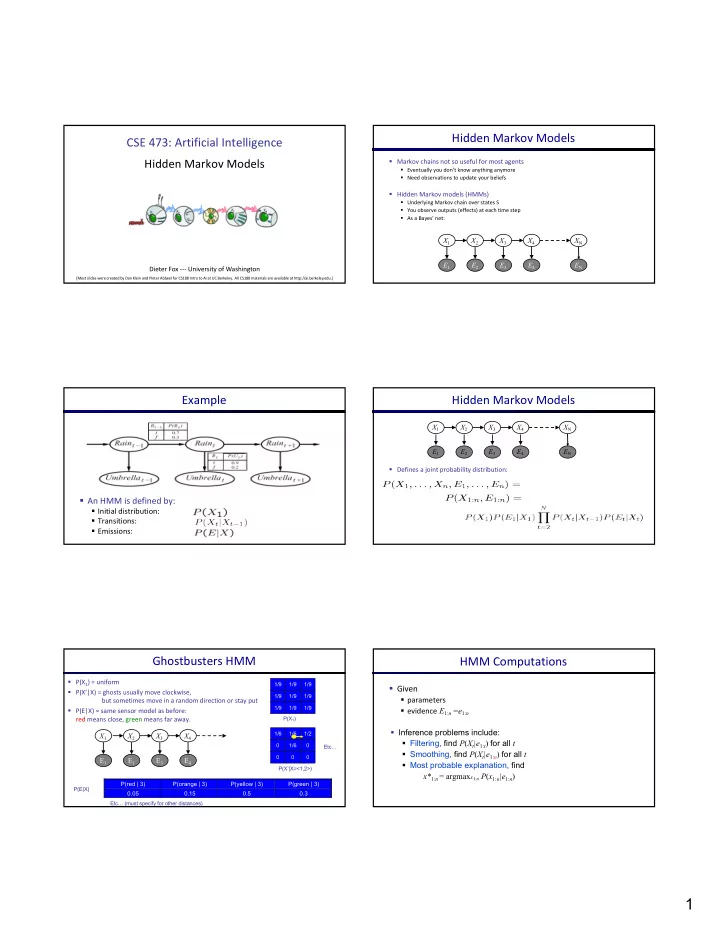

Hidden Markov Models CSE 473: Artificial Intelligence Hidden Markov Models § Markov chains not so useful for most agents § Eventually you don’t know anything anymore § Need observations to update your beliefs § Hidden Markov models (HMMs) § Underlying Markov chain over states S § You observe outputs (effects) at each time step § As a Bayes’ net: X 1 X 2 X 3 X 4 X N X 5 E 1 E 2 E 3 E 4 E N E 5 Dieter Fox --- University of Washington [Most slides were created by Dan Klein and Pieter Abbeel for CS188 Intro to AI at UC Berkeley. All CS188 materials are available at http://ai.berkeley.edu.] Example Hidden Markov Models X 1 X 2 X 3 X 4 X N X 5 E 1 E 2 E 3 E 4 E N E 5 § Defines a joint probability distribution: § An HMM is defined by: § Initial distribution: § Transitions: § Emissions: Ghostbusters HMM HMM Computations § P(X 1 ) = uniform 1/9 1/9 1/9 § Given § P(X’|X) = ghosts usually move clockwise, 1/9 1/9 1/9 § parameters but sometimes move in a random direction or stay put 1/9 1/9 1/9 § evidence E 1: n =e 1: n § P(E|X) = same sensor model as before: red means close, green means far away. P(X 1 ) § Inference problems include: 1/6 1/6 1/2 X 1 X 2 X 3 X 4 § Filtering, find P ( X t |e 1: t ) for all t 0 1/6 0 Etc… § Smoothing, find P ( X t |e 1: n ) for all t 0 0 0 E 1 E 1 E 3 E 4 § Most probable explanation, find P(X’|X=<1,2>) x* 1: n = argmax x 1: n P ( x 1: n |e 1: n ) P(red | 3) P(orange | 3) P(yellow | 3) P(green | 3) E 5 P(E|X) 0.05 0.15 0.5 0.3 Etc… (must specify for other distances) 1
Real HMM Examples Real HMM Examples § Speech recognition HMMs: § Machine translation HMMs: § Observations are acoustic signals (continuous valued) § Observations are words (tens of thousands) § States are specific positions in specific words (so, tens of thousands ) § States are translation options X 1 X 2 X 3 X 4 X 1 X 2 X 3 X 4 E 1 E 1 E 3 E 4 E 1 E 1 E 3 E 4 Real HMM Examples Conditional Independence § HMMs have two important independence properties: § Robot tracking: § Markov hidden process, future depends on past via the present § Observations are range readings (continuous) ? ? § States are positions on a map (continuous) X 1 X 2 X 3 X 4 X 1 X 2 X 3 X 4 E 1 E 1 E 3 E 4 E 1 E 1 E 3 E 4 Conditional Independence Conditional Independence § HMMs have two important independence properties: § HMMs have two important independence properties: § Markov hidden process, future depends on past via the present § Markov hidden process, future depends on past via the present § Current observation independent of all else given current state § Current observation independent of all else given current state ? X 1 X 2 X 3 X 4 X 1 X 2 X 3 X 4 E 1 E 1 E 3 E 4 E 1 E 1 E 3 E 4 ? ? ? § Quiz: does this mean that observations are independent given no evidence? § [No, correlated by the hidden state] 2
Filtering / Monitoring Example: Robot Localization Example from § Filtering, or monitoring, is the task of tracking the distribution B(X) (the belief state) Michael Pfeiffer over time § We start with B(X) in an initial setting, usually uniform § As time passes, or we get observations, we update B(X) § The Kalman filter (one method – Real valued values) Prob 0 1 § invented in the 60’s as a method of trajectory estimation for the Apollo program t=0 Sensor model: can read in which directions there is a wall, never more than 1 mistake Motion model: may not execute action with small prob. Example: Robot Localization Example: Robot Localization Prob 0 1 Prob 0 1 t=1 Lighter grey: was possible to get the reading, but less likely b/c t=2 required 1 mistake Example: Robot Localization Example: Robot Localization Prob 0 1 Prob 0 1 t=3 t=4 3
Example: Robot Localization Inference Recap: Simple Cases X 1 X 1 X 2 E 1 Prob 0 1 t=5 Passage of Time Online Belief Updates § Assume we have current belief P(X | evidence to date) § Every time step, we start with current P(X | evidence) § We update for time: X 1 X 2 X 1 X 2 § Then, after one time step passes: § Or, compactly: § We update for evidence: X 2 E 2 § Basic idea: beliefs get “pushed” through the transitions § The forward algorithm does both at once (and doesn’t normalize) § With the “B” notation, we have to be careful about what time step t the belief is about, and § Problem: space is |X| and time is |X| 2 per time step what evidence it includes Observation Example: Passage of Time § As time passes, uncertainty “accumulates” § Assume we have current belief P(X | previous evidence): X 1 § Then: E 1 § Or: T = 1 T = 2 T = 5 § Basic idea: beliefs reweighted by likelihood of evidence § Unlike passage of time, we have to renormalize Transition model: ghosts usually go clockwise 4
Example: Observation The Forward Algorithm § As we get observations, beliefs get reweighted, uncertainty § We want to know: “decreases” § We can derive the following updates Before observation After observation § To get , compute each entry and normalize Example: Run the Filter Example HMM § An HMM is defined by: § Initial distribution: § Transitions: § Emissions: Courtesy of T. Choudhury, G. Borriello Summary: Filtering Intel Multi-Sensor Board § Filtering is the inference process of finding a distribution over X T given e 1 through e T : P( X T | e 1:t ) § We first compute P( X 1 | e 1 ): § For each t from 2 to T, we have P( X t-1 | e 1:t-1 ) § Elapse time: compute P( X t | e 1:t-1 ) § Observe: compute P(X t | e 1:t-1 , e t ) = P( X t | e 1:t ) Dieter Fox, University of 30 Washington 5
New device New device Dieter Fox, University of Washington 31 Dieter Fox, University of Washington 32 Activity Model Courtesy of T. Choudhury, G. Borriello [UAI-06, ISER-06] Sensor board: Data Stream e t-1 e t Environment indoor, outdoor, vehicle Activity a t-1 a t walk, run, stop, up/downstairs, drive, elevator, cover c t-1 c t Boosted classifier outputs [Choudhury et al., IJCAI-05] Dieter Fox, University of 33 Washington After Action Review Evaluation (DARPA/NIST) 6
Best Explanation Queries State Path Trellis § State trellis: graph of states and transitions over time sun sun sun sun X 1 X 2 X 3 X 4 X 5 rain rain rain rain E 1 E 2 E 3 E 4 E 5 § Each arc represents some transition § Each arc has weight § Query: most likely seq: § Each path is a sequence of states § The product of weights on a path is the seq’s probability § Can think of the Forward (and now Viterbi) algorithms as computing sums of all paths (best paths) in this graph Viterbi Algorithm Example sun sun sun sun rain rain rain rain 22 23 Recap: Reasoning Over Time 0.3 § Stationary Markov models 0.7 rain sun X 1 X 2 X 3 X 4 0.7 0.3 § Hidden Markov models X E P rain umbrella 0.9 X 1 X 2 X 3 X 4 X 5 rain no umbrella 0.1 sun umbrella 0.2 E 1 E 2 E 3 E 4 E 5 sun no umbrella 0.8 7
Recommend
More recommend