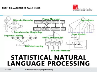
Statistical Natural Language Processing Prasad Tadepalli CS430 - PDF document

Statistical Natural Language Processing Prasad Tadepalli CS430 lecture Natural Language Processing Some subproblems are partially solved – Spelling correction, grammar checking – Information retrieval with keywords – Semi-automatic translation in narrow domains, e.g., travel planning – Information extraction in narrow domains – Speech recognition 1

Challenges • Common-sense reasoning • Language understanding at a deep level • Semantics-based information retrieval • Knowledge representation and inference • A model of learning semantics or meaning • Robust learning of grammars Language Models • Unigram models For every word w , learn the prior P(w) • Bigram models For every word pair, (W i , W j ) learn the probability of W j following W i : P(W j | W i ) • Trigram models: P(W k | W i , W j ) probability of W k following W i and W j . Of None of these sufficiently capture grammar! 2

Context-free Grammars • Variables – Noun Phrase, Verb Phrase, Noun, Verb etc. • Terminals (words) – Book, a, smells, wumpus, the, etc. • Production Rules – [Sentence] -> [Noun Phrase] [Verb Phrase] – [Noun Phrase] -> [Article] [Noun] – [Verb Phrase] -> [Verb] [Noun Phrase] • Start Symbol: [Sentence] Parse Tree Sentence Noun Phrase Verb Phrase Article Noun Verb The Wumpus Smells Natural language is ambiguous – needs a “softer” grammar. 3

Probabilistic CFGs • Context-free grammars with probabilities attached to each production • The probabilities of different productions with the same left hand side sum to 1 • Semantics: the conditional probability of a variable generating the right hand side [Noun Phrase] -> [Noun] (0.1) | [Article] [Noun] (0.8)| [Article] [Adjective] [Noun] (0.1) Learning PCFGs • From Sentences and their parse trees: Counting: Count the number of times each variable occurs in the parse trees and generates each possible r.h.s. #of times A-> rhs occurs Probability= ---------------------------------- #of times A occurs 4

Inside-Outside Algorithm • Applicable when parse trees are not given • An instance of the EM Algorithm: treat the parse trees as “hidden variables” of EM –Start with an intial random PCFG –Repeat until convergence • E-step: Estimate the probability that each subsequence is generated by each rule • M-step: Estimate the probability of each rule Information Retrieval • Given a query, how to retrieve documents that answers the query? • So far semantics-based methods are not as successful as word-based methods • The documents and the query are treated as bags of words, disregarding the syntax. • Stemming (removing suffixes like “ing”) and “stop words” (eg, “the”) removal are found useful. 5

Vector Space Model • TF-IDF computed for each word-doc pair • There are many versions of this measure • TF is the term frequency: the number of times a term (word) occurs in the doc • IDF is “inverse document frequency” of the word = log(|D|/DF(w)), where DF(w) is the number of documents in which w occurs and D is the set of all documents. • Common words like “all” “the” etc. have high document frequency and low IDF Rocchio Method • Each document is described as a vector in an n-dimensional space, where each dimension represents a term Doc1 = [t(1,1),t(1,2),…,t(1,n)] Doc2 = [t(2,1),t(2,2),…,t(2,n)] t[I,j] is the tf-idf of document i and term j . • Two vectors are similar if their cosine distance (normalized dot product) is small. 6

Cosine Distance • Doc1 = [t(1,1),t(1,2),…,t(1,n)] Doc2 = [t(2,1),t(2,2),…,t(2,n)] • CosineDistance(Doc1,Doc2) = + + t ( 1 , 1 ) * t ( 2 , 1 ) .... t ( 1 , n ) * t ( 2 , n ) 2 2 2 2 + + + + t ( 1 , 1 ) ... ... t ( 1 , n ) t ( 2 , 1 ) t ( 2 , n ) • The documents are ranked by their cosine distance to the query, treated as another document Naïve Bayes • Naïve Bayes is very effective for document retrieval • Naïve Bayes assumes that the features X are independent, given the class Y • Medical diagnosis: Class Y = disease Features X = symptoms • Information retrieval: Class Y = document Features X = words 7

Naïve Bayes for Retrieval • Build a unigram model for each document: Estimate P( W j |D i ) for each document D i and W j (easily done by counting). • Each document D i has a prior probability P(D i ) of being relevant regardless of any query, e.g., today’s newspaper has much higher prior than, say, yesterday’s paper. Naïve Bayes for Retrieval • The posterior probability of a document’s relevance given the query is P(D i |W 1 …W n ) = α P(D i ) P(W 1 …W n |D i ) [ Bayes Rule] = α P(D i ) P(W 1 | D i ) … P(W n | D i ) [conditional independence of features] where α is a normalizing factor and the same for all documents (so ignored) • To avoid zero probabilities, a pseudo- count of 1 is added for each W j - D i pair (Laplace correction) 8

Evaluating IR Systems Relevant Not relevant Retrieved 15 10 Not retrieved 20 55 Accuracy = (15+55)/100 = 70%. It is misleading! Accuracy if no docs are retrieved = 65%. Recall = number of retrieved docs as a percentage of relevant documents =15/35 = 43% Precision = number of relevant docs as a percentage of retrieved documents =15/25 = 60% Precision Recall Curves We want high precision and high recall. Usually there is a controllable parameter that can tradeoff one against the other 100 Precision 50 0 50 100 0 Recall 9