Recent advances in fluid boundary layer theory Anne-Laure Dalibard - PowerPoint PPT Presentation

Recent advances in fluid boundary layer theory Anne-Laure Dalibard (Sorbonne Universit´ e, Paris) M ∩ Φ - ICMP 2018 July 25th, 2018 - Montreal

Outline The Prandtl boundary layer equation The stationary case The time-dependent case

The Prandtl boundary layer equation Plan The Prandtl boundary layer equation The stationary case The time-dependent case

The Prandtl boundary layer equation Fluids with small viscosity Goal: understand the behavior of 2d fluids with small viscosity in a domain Ω ⊂ R 2 . ∂ t u ν + ( u ν · ∇ ) u ν + ∇ p ν − ν ∆ u ν = 0 in Ω , div u ν = 0 in Ω , (1) u ν u ν | t =0 = u ν | ∂ Ω = 0 , ini . → Singular perturbation problem. Formally, if u ν → u E , and if ∆ u ν remains bounded, then u E is a solution of the Euler system ∂ t u E + ( u E · ∇ ) u E + ∇ p E = 0 in Ω , (2) div u ν = 0 in Ω . But what about boundary conditions?

The Prandtl boundary layer equation Boundary conditions • Navier-Stokes: parabolic system. → Dirichlet boundary conditions can be enforced: u ν | ∂ Ω = 0. • Euler: ∼ hyperbolic system, with a divergence-free condition div u E = 0. → Condition on the normal component only (non-penetration condition): u E · n | ∂ Ω = 0. Consequence: ◮ Loss of the tangential boundary condition as ν → 0; ◮ Formation of a boundary layer in the vicinity of ∂ Ω to correct the mismatch between 0(= u ν · τ | ∂ Ω ) and u E · τ | ∂ Ω . p i ee

The Prandtl boundary layer equation The whole space case Theorem [Constantin& Wu, ’96] If Ω = R 2 or Ω = T 2 , any family of Leray-Hopf solutions u ν ∈ C ( R + , L 2 ) ∩ L 2 ( R + , H 1 ) of the Navier-Stokes system converges as ν → 0 towards a solution of the Euler system. Proof: energy estimate, by considering u E as a solution of Navier-Stokes with a remainder − ν ∆ u E . Consequence: if convergence fails, problems come from the boundary.

The Prandtl boundary layer equation The half-space case: Prandtl’s Ansatz Prandtl, 1904: in the limit ν ≪ 1, if Ω = R 2 + , u E ( x , y ) for y ≫ √ ν (sol. of 2d Euler), � u ν ( x , y ) ≃ � u P � � , √ ν v P � �� for y � √ ν. y y x , x , √ ν √ ν The velocity field ( u P , v P ) satisfies the Prandtl system ∂ t u P + u P ∂ x u P + v P ∂ Y u P − ∂ YY u P = − ∂ p E ∂ x ( t , x , 0) ∂ x u P + ∂ Y v P = 0 , u P Y →∞ u P ( x , Y ) = u ∞ ( t , x ) := u E ( t , x , 0) , | Y =0 = 0 , lim u P | t =0 = u P ini .

The Prandtl boundary layer equation The Prandtl equation: general remarks ∂ t u P + u P ∂ x u P + v P ∂ Y u P − ∂ YY u P = − ∂ p E ∂ x ( t , x , 0) ∂ x u P + ∂ Y v P = 0 , (P) u P Y →∞ u P ( x , Y ) = u ∞ ( t , x ) := u E ( t , x , 0) , | Y =0 = 0 , lim u P | t =0 = u P ini . Comments: � Y ◮ Nonlocal, scalar equation: write v P = − 0 u P x ; ◮ Pressure is given by Euler flow= data; ◮ Main source of trouble: nonlocal transport term v P ∂ Y u P (loss of one derivative).

The Prandtl boundary layer equation Questions around the Prandtl system 1. Is the Prandtl system well-posed? (i.e. does there exist a unique solution?) In which functional spaces? Under which conditions on the initial data? 2. When the Prandtl system is well-posed, can we justify the Prandtl Ansatz? i.e. can we prove that � u ν − u ν app � → 0 as ν → 0 in some suitable functional space, where the function u ν app is such that u E ( x , y ) for y ≫ √ ν � u ν � u P � � , √ ν v P � �� for y � √ ν. app ( x , y ) ≃ y y x , x , √ ν √ ν

The Prandtl boundary layer equation Functional spaces �� Ω | u | 2 � 1 / 2 . • L 2 space: � u � L 2 (Ω) = • Sobolev spaces H s , s ∈ N: � u � H s = � | k |≤ s �∇ k u � L 2 . • Space of analytic functions: ∃ C > 0, s.t. for all k ∈ N d , |∇ k u ( x ) | ≤ C | k | +1 | k | ! . sup x ∈ Ω • Gevrey spaces G τ , τ > 0 : ∃ C > 0, s.t. for all k ∈ N d , |∇ k u ( x ) | ≤ C | k | +1 ( | k | !) τ . sup x ∈ Ω If τ > 1, G τ contains non trivial functions with compact support.

The stationary case Plan The Prandtl boundary layer equation The stationary case The time-dependent case

The stationary case Well-posedness under positivity assumptions Stationary Prandtl system: u ∂ x u + v ∂ Y u − ∂ YY u = − ∂ p E ∂ x ( x , 0) (SP) ∂ x u + ∂ Y v = 0 , u | x =0 = u 0 u | Y =0 = 0 , v | Y =0 = 0 , Y →∞ u ( x , Y ) = u ∞ ( x ) . lim ∼ Non-local, “transport-diffusion” equation . Theorem [Oleinik, 1962]: Let u 0 ∈ C 2 ,α ( R + ) , α > 0 . Assume that b u 0 ( Y ) > 0 for Y > 0 , u ′ 0 (0) > 0 , u ∞ > 0 , and that − ∂ YY u 0 + ∂ p E ∂ x (0 , 0)) = O ( Y 2 ) for 0 < Y ≪ 1 . Then there exists x ∗ > 0 such that (SP) has a unique strong C 2 solution in { ( x , Y ) ∈ R 2 , 0 ≤ x < x ∗ , 0 ≤ Y } . If ∂ p E ( x , 0) ≤ 0 , ∂ x then x ∗ = + ∞ .

The stationary case Well-posedness under positivity assumptions Stationary Prandtl system: u ∂ x u + v ∂ Y u − ∂ YY u = − ∂ p E ∂ x ( x , 0) (SP) ∂ x u + ∂ Y v = 0 , u | x =0 = u 0 u | Y =0 = 0 , v | Y =0 = 0 , Y →∞ u ( x , Y ) = u ∞ ( x ) . lim ∼ Non-local, “transport-diffusion” equation . Theorem [Oleinik, 1962]: Let u 0 ∈ C 2 ,α ( R + ) , α > 0 . Assume that b u 0 ( Y ) > 0 for Y > 0 , u ′ 0 (0) > 0 , u ∞ > 0 , and that − ∂ YY u 0 + ∂ p E ∂ x (0 , 0)) = O ( Y 2 ) for 0 < Y ≪ 1 . Then there exists x ∗ > 0 such that (SP) has a unique strong C 2 solution in { ( x , Y ) ∈ R 2 , 0 ≤ x < x ∗ , 0 ≤ Y } . If ∂ p E ( x , 0) ≤ 0 , ∂ x then x ∗ = + ∞ .

The stationary case Comments on Oleinik’s theorem ◮ The solution lives as long as there is no recirculation, i.e. as long as u remains positive. ◮ Proof relies on a nonlinear change of variables [von Mises]: transforms (SP) into a local diffusion equation (porous medium type). → Maximum principle holds for the new eq. by standard tools and arguments. ◮ Maximal existence “time” x ∗ : if x ∗ < + ∞ , then (i) either ∂ Y u ( x ∗ , 0) = 0 (ii) or ∃ Y ∗ > 0 , u ( x ∗ , Y ∗ ) = 0. ◮ Monotony (in Y ) is preserved by the equation. If u 0 is monotone, scenario (ii) cannot happen.

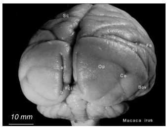
The stationary case Illustration of the “separation” phenomenon Ë ië Ë il ∂ u Separation point: ∂ Y | x = x ∗ , Y =0 = 0 . Figure: Cross-section of a flow past a cylinder (source: ONERA, France)

The stationary case Goldstein singularity ◮ Formal computations of a solution by [Goldstein ’48, Stewartson ’58] (asymptotic expansion in well-chosen self-similar variables). Prediction: there exists a solution such that ∂ Y u | Y =0 ( x ) ∼ √ x ∗ − x as x → x ∗ . Heuristic argument by Landau giving the same separation rate. ◮ [D., Masmoudi, ’18]: rigorous justification of the Goldstein singularity. Computation of an approximate solution, using modulation of variables techniques. Open problem: is √ x ∗ − x the “stable” separation rate? ◮ Why “singularity”? � Y 0 u x , v becomes infinite as x → x ∗ : separation. Since v = − ◮ In this case, “generically”, recirculation causes separation.

The stationary case Goldstein singularity ◮ Formal computations of a solution by [Goldstein ’48, Stewartson ’58] (asymptotic expansion in well-chosen self-similar variables). Prediction: there exists a solution such that ∂ Y u | Y =0 ( x ) ∼ √ x ∗ − x as x → x ∗ . Heuristic argument by Landau giving the same separation rate. ◮ [D., Masmoudi, ’18]: rigorous justification of the Goldstein singularity. Computation of an approximate solution, using modulation of variables techniques. Open problem: is √ x ∗ − x the “stable” separation rate? ◮ Why “singularity”? � Y 0 u x , v becomes infinite as x → x ∗ : separation. Since v = − ◮ In this case, “generically”, recirculation causes separation.

The stationary case Goldstein singularity ◮ Formal computations of a solution by [Goldstein ’48, Stewartson ’58] (asymptotic expansion in well-chosen self-similar variables). Prediction: there exists a solution such that ∂ Y u | Y =0 ( x ) ∼ √ x ∗ − x as x → x ∗ . Heuristic argument by Landau giving the same separation rate. ◮ [D., Masmoudi, ’18]: rigorous justification of the Goldstein singularity. Computation of an approximate solution, using modulation of variables techniques. Open problem: is √ x ∗ − x the “stable” separation rate? ◮ Why “singularity”? � Y 0 u x , v becomes infinite as x → x ∗ : separation. Since v = − ◮ In this case, “generically”, recirculation causes separation.

The stationary case Open problems for the stationary case ◮ Remove Goldstein singularity by adding corrector terms in the equation, coming from the coupling with the outer flow (triple deck system?); ◮ Construct solutions with recirculation.