Random Variable : non empty set. {up, town} Event A: is a subset - PDF document
Introduction to Probability and Hidden Markov Models Durbin et al. Ch3 EECS 458 CWRU Fall 2004 Random Variable : non empty set. {up, town} Event A: is a subset of . {up} A random variable X is a function defined on events
Introduction to Probability and Hidden Markov Models Durbin et al. Ch3 EECS 458 CWRU Fall 2004 Random Variable • Ω : non empty set. {up, town} • Event A: is a subset of Ω . {up} • A random variable X is a function defined on events with range in a subset of R . X ({up})=1, X ({down})=0. • The probability of an event A, denoted as P (A), is the likelihood of the occurrence of A. It is a function that maps events to [0,1] that satisfies the following conditions: sum( P (A)) = 1. For example: P ({up}) = P ({down}) = 0.5. • The distribution function of a r.v. is defined as the probability function. Examples • A die with 4 sides labeled using A, C, G, T. The probability of each letter x ∈ { A, C, G, T } that occurs in a roll is p x . • The probability of a sequence of “AAGC” is generated by the simple model is just p A * p A * p G * p C . 1
Conditional probability • The joint probability of two events A and B (P(A,B)) is the probability that event A and B occur at the same time. • The conditional probability of P(B|A) is the probability that B occurs given A occurred. • Facts: – P(B|A) = P( AB)/P(A) – P(A) = ∑ i P(AB i )= ∑ i P(A|B i )P(B i ) An example • A family has two children, sample space: Ω = {GG,BB,BG,GB} • P(GG)=P(BB)=P(BG)=P(GB)=0.25 • ? P(BB|1 boy at least) • ? P(BB|older is a boy) Bayes Theorem Bayes Theorem: P(B|A) = P(AB)/P(A) =(P(A|B)P(B))/ ∑ i P(AC i )= ∑ i P(A|C i )P(C i ) Two events are independent if P(AB) = P( A)P(B), i.e. P(B|A) = P(B) Example: playing card, the suit and the rank. P(King)=4/52=1/13, P(King|Spade)=1/13 2
Expectation of a r.v. • E(X) := ∑ xP(X=x) • E(g(X))= ∑ g(x)P(X=x) • E(aX+bY) = aE(X)+bE(Y) • E(XY)=E(X)E(Y) if X and Y are independent • Var(X) := E((X-EX) 2 ) = EX 2 -(EX) 2 • Var(aX)=a 2 Var(X) Roadmap • Model selection • Model inference • Markov models • Hidden Markov models • Applications Probabilistic models • A model is a mathematical formulation that explains/simulates the data under consideration. • Linear model: – Y=aX+b – Y=aX+b+ ε , where ε is a r.v. • Generating models for bio sequences 3
Model selection • Everything else being equal, one should prefer simpler one. • Should take into consideration background/prior knowledge of the problem. • Some explicit measure can be used, such as minimum description length (MDL). Minimum Description Length • Connections to information theory, communication channels and data compression • Prefer models that minimize the length of the message required to describe the data. Minimum Description Length • The most probable model is also the one with the shortest description. • The “better” the model, the shortest the message describing the observation x, the highest the compression (and vice versa) • Keep in mind that if the model is too faithful on the observation, it could lead to over fitting and has poor generalization. 4
Model inference • Once a model is fixed, parameters need to be estimated from data. • Two views: – True parameters are fixed values in a space, we need to find them. Classical /Frequencist – Parameters themselves are r.v.s and we need to estimate their distributions. Bayesian. Maximum likelihood • Given a model M with some unknown parameters θ , and some training data set x , the maximum likelihood estimate of θ is θ ML = argmax θ P(x|M, θ ) where the P(x|M, θ ) is the probability that the dataset x has been generated by the model M with parameters θ . • MLE is consistent estimate, i.e. , if we have enough data, the MLE is close to the true value. • With small dataset, overfitting, Example • Two dice with four faces: {A,C,G,T} • One has the distribution of p A = p C = p G = p T =0.25 • The other has the distribution: p A =0.20, p C =0.28, p G =0.30, p T =0.22 5
Example: generating model • The source generates a string as follows: 1. Randomly select one die with the probability distribution of p 1 =0.9, p 2 =0.1. 2. Roll it, append the symbol to the string. 3. Repeat 1-2, until all symbols have been generated. Parameter θ : {0.9*{0.25, 0.25, 0.25, 0.25,}, 0.1*{0.20,0.28,0.30,0.22}} Example • Suppose we don’t know the model, neither the parameters • Given a string generated by the unknown model, say x=“GATTCCAA…” • Questions: – How to choose a “good” model? – How to infer parameters? – How much data do we need? Bernoulli and Markov models • There are two typical hypothesis about the source • Bernoulli: symbols are generated independently and they are identically distributed (iid) • Markov: the probability distribution for the “next” symbol depends on the previous h symbols ( h >0 is the order of Markov chain). 6
Example • X1 = CCACCCTTGT • X2 = TTGTTCTTCC • X3 = TTCAACCGGT • X4 = AATAACCCCA • MLE for the parameter set { p A , p C , p G , p T } for Bernoulli model is: p A =8/40=0.20, p C =15/40=0.375, p G =4/40=0.10, p T =13/40=0.325 Issues • How can we incorporate prior knowledge in the analysis process? • Over fitting • How can we compare different models? Bayesian inference • Useful to get better estimates of the parameters using prior knowledge • Useful to compare different models • Parameters themselves are r.v.s. Prior knowledge represented by prior distribution of parameters. We need to estimate the posterior distribution of parameters given data. 7
Bayesian inference θ θ ( | ) ( ) P x P θ = ( | ) P x ∫ δ δ ( | ) P x d Point estimation • We can define the “best” model as the one that maximizes P ( θ |x) (mazimum a posteriori estimation, or MAP). • Equivalent to minimize: -log P ( θ |x) = -log P (x| θ ) – log P ( θ ) +log P (x) • Can be used for model comparisons • Note that log P (x) can be regarded as a constant ML and MAP • ML estimation: θ ML = argmax θ P(x| θ ) θ ML = argmin θ {-log P(x| θ ) } • MAP estimation: θ MAP = argmin θ {-log P(x| θ )-log θ )} 8
Occam’s Razor • Everything else being equal, one should prefer a simple model over a complex one • One can incorporate this principle in the Bayesian framework by using priors which penalize complex models. Example • Two dice with four faces: {A,C,G,T} • One has the distribution of p A = p C = p G = p T =0.25. M1 • The other has the distribution: p A =0.20, p C =0.28, p G =0.30, p T =0.22. M2 Example • The source generates a string as follows: 1. Randomly select one die. 2. Roll it, append the symbol to the string. 3. Repeat 2, until all symbols have been generated. – Given a string say x=“GATTCCAA…” 9
Example (ML) • What is the probability of the data is generated by M1? M2? • P(x|M1) • P(x|M2) • They can be easily calculated since this is a Bernoulli model. • Log Likelihood Ratio: log(P(x|M1))- log(P(x|M2)) Example • Which die or model is selected in step 1? What is the probability distribution of selecting model 1 and model 2. • Prior: if we know nothing, better assume they are equally likely to be selected. But in some case, we know sth. Say P(M1) =0.4, P(M2) = 0.6. • Given the data (x=“GATTCCAA…”), what can we say about the question? Example (Bayesian) • P(M1|x) = P(x|M1)P(D1)/P(x) • P(M2|x) = P(x|M2)P(D2)/P(x) • This is the posterior distribution. We can choose the model using MAP criterion. 10
Markov models • Recall that in general we assume a sequence is generated by a source/model. • For Bernoulli models, each letter is independent generated. • For Markov models, the generation of the current letter depends on the previous letters, i.e., what we are going to see depends on what we have seen. Markov models (Markov chain) • Order h ; how many previous steps • States, correspond to letters (for current moment) • Transition probabilities : p x,y the probability of generating y given we have seen x . • Stationary probability: the limit distribution of the state probabilities. First order MM = = ( | ... ) ( | ) P a a a a P a a p − − − 1 2 1 1 , m m m m m a a − 1 m m = P ( a a a ... a ) P ( a | a a ... a ) P ( a a ... a ) − − − − − − m m 1 m 2 1 m m 1 m 2 1 m 1 m 2 1 = ( | ) ( | )... ( | ) ( ) P a a P a a P a a P a − − − 1 1 2 2 1 1 m m m m ∏ = ( ) p P a a , a 1 − i 1 i 11
First order MM A C b e G T Transition probability b A C G T e b 0.25 0.25 0.25 0.25 A 0.1 0.1 0.3 0.3 0.2 C 0.2 0.2 0.2 0.3 0.1 G 0.3 0.3 0.2 0.15 0.05 T 0.15 0.15 0.4 0.25 0.05 e Example: CpG islands • CpG islands are stretches of C and G bases repeating over and over • Often occur adjacent to gene-rich areas, forming a barrier between the genes and “junk” DNA • It is important to identify CpG islands for gene recognition. 12
Recommend
More recommend
Explore More Topics
Stay informed with curated content and fresh updates.
