Quick Warm-Up Suppose we have a biased coin that comes up heads with - PowerPoint PPT Presentation

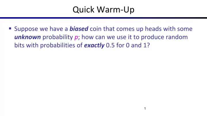
Quick Warm-Up  Suppose we have a biased coin that comes up heads with some unknown probability p ; how can we use it to produce random bits with probabilities of exactly 0.5 for 0 and 1? 1

Quick Warm-Up  Suppose we have a biased coin that comes up heads with some unknown probability p ; how can we use it to produce random bits with probabilities of exactly 0.5 for 0 and 1?  Answer (von Neumann):  Flip coin twice, repeat until the outcomes are different  HT = 0, TH = 1, each has probability p (1- p ) 2

Bayes Nets Part I: Representation Part II: Exact inference  Enumeration (always exponential complexity)  Variable elimination (worst-case exponential complexity, often better)  Inference is NP-hard in general Part III: Approximate Inference Later: Learning Bayes nets from data

CS 188: Artificial Intelligence Bayes Nets: Approximate Inference Instructors: Sergey Levine and Stuart Russell University of California, Berkeley

Sampling  Why sample?  Often very fast to get a decent  Basic idea approximate answer  Draw N samples from a sampling distribution S  The algorithms are very simple and  Compute an approximate posterior probability general (easy to apply to fancy models)  They require very little memory (O(n))  Show this converges to the true probability P  They can be applied to large models, whereas exact algorithms blow up

Example  Suppose you have two agent programs A and B for Monopoly  What is the probability that A wins?  Method 1:  Let s be a sequence of dice rolls and Chance and Community Chest cards  Given s , the outcome V ( s ) is determined (1 for a win, 0 for a loss) ∑ s P ( s ) V ( s )  Probability that A wins is  Problem: infinitely many sequences s !  Method 2:  Sample N sequences from P ( s ) , play N games (maybe 100)  Probability that A wins is roughly 1/ N ∑ i V ( s i ) i.e., fraction of wins in the sample 6

Sampling basics: discrete ( categorical ) distribution  Example  To simulate a biased d-sided coin:  Step 1: Get sample u from uniform C P(C) distribution over [0, 1) 0.0 ≤ u < 0.6, → C=red  E.g. random() in python red 0.6 0.6 ≤ u < 0.7, → C=green  Step 2: Convert this sample u into an green 0.1 0.7 ≤ u < 1.0, → C=blue outcome for the given distribution by blue 0.3 associating each outcome x with a P ( x )-sized sub-interval of [0,1)  If random() returns u = 0.83, then the sample is C = blue  E.g, after sampling 8 times:

Sampling in Bayes Nets  Prior Sampling  Rejection Sampling  Likelihood Weighting  Gibbs Sampling

Prior Sampling

Prior Sampling P ( C ) c 0.5 ¬ c 0.5 P ( S | C ) P ( R | C ) Cloudy Cloudy s 0.1 r 0.8 c c ¬ s ¬ r 0.9 0.2 ¬ c ¬ c s 0.5 r 0.2 Sprinkler Sprinkler Rain Rain ¬ s ¬ r 0.5 0.8 P ( W | S,R ) Samples: WetGrass WetGrass w 0.99 r s c, ¬ s, r, w ¬ w 0.01 ¬ c, s, ¬ r, w ¬ r w 0.90 ¬ w 0.10 … w 0.90 ¬ s r ¬ w 0.10 ¬ r w 0.01 ¬ w 0.99

Prior Sampling  For i=1, 2, …, n (in topological order)  Sample X i from P( X i | parents ( X i ))  Return ( x 1 , x 2 , …, x n )

Prior Sampling  This process generates samples with probability: ∏ i P ( x i | parents ( X i )) = P ( x 1 ,…, x n ) S PS ( x 1 ,…, x n ) = …i.e. the BN ’ s joint probability  Let the number of samples of an event be N PS ( x 1 ,…, x n )  Estimate from N samples is Q N ( x 1 ,…, x n ) = N PS ( x 1 ,…, x n )/ N  Then lim N → ∞ Q N ( x 1 ,…, x n ) = lim N →∞ N PS ( x 1 ,…, x n )/ N = S PS ( x 1 ,…, x n ) = P ( x 1 ,…, x n )  I.e., the sampling procedure is consistent

Example  We’ll get a bunch of samples from the BN: C c, ¬ s, r, w c, s, r, w S R ¬ c, s, r, ¬ w W c, ¬ s, r, w ¬ c, ¬ s, ¬ r, w  If we want to know P( W )  We have counts <w:4, ¬ w:1>  Normalize to get P( W ) = <w:0.8, ¬ w:0.2>  This will get closer to the true distribution with more samples  Can estimate anything else, too  E.g., for query P( C | r, w ) use P( C | r, w ) = α P( C , r, w )

Rejection Sampling

Rejection Sampling  A simple modification of prior sampling for conditional probabilities  Let’s say we want P( C | r, w ) C  Count the C outcomes, but ignore (reject) S R samples that don’t have R =true, W =true W  This is called rejection sampling  It is also consistent for conditional c, ¬ s, r, w probabilities (i.e., correct in the limit) c, s, ¬ r ¬ c, s, r, ¬ w c, ¬ s, ¬ r ¬ c, ¬ s, r, w

Rejection Sampling  Input: evidence e 1 ,.., e k  For i=1, 2, …, n  Sample X i from P( X i | parents ( X i ))  If x i not consistent with evidence  Reject: Return, and no sample is generated in this cycle  Return (x 1 , x 2 , …, x n )

Likelihood Weighting

Likelihood Weighting  Problem with rejection sampling:  Idea: fix evidence variables, sample the rest  If evidence is unlikely, rejects lots of samples  Problem: sample distribution not consistent!  Evidence not exploited as you sample  Solution: weight each sample by probability of evidence variables given parents  Consider P( Shape | Color=blue ) pyramid, blue pyramid, green pyramid, blue pyramid, red sphere, blue sphere, blue Shape Color Shape Color cube, blue cube, red sphere, blue sphere, green

Likelihood Weighting P ( C ) c 0.5 ¬ c 0.5 P ( S | C ) P ( R | C ) Cloudy Cloudy s 0.1 r 0.8 c c ¬ s ¬ r 0.9 0.2 ¬ c ¬ c s 0.5 r 0.2 Sprinkler Sprinkler Rain Rain ¬ s ¬ r 0.5 0.8 P ( W | S,R ) Samples: WetGrass WetGrass w 0.99 r s ¬ w x 0.1 x 0.99 c , s, , w r w = 1.0 0.01 ¬ r w 0.90 ¬ w 0.10 w 0.90 ¬ s r ¬ w 0.10 ¬ r w 0.01 ¬ w 0.99

Likelihood Weighting  Input: evidence e 1 ,.., e k  w = 1.0  for i=1, 2, …, n  if X i is an evidence variable  x i = observed value i for X i  Set w = w * P(x i | Parents(X i ))  else  Sample x i from P(X i | Parents(X i ))  return (x 1 , x 2 , …, x n ), w

Likelihood Weighting  Sampling distribution if Z sampled and e fixed evidence S WS ( z , e ) = ∏ i P ( z i | parents ( Z i )) Cloudy C S R  Now, samples have weights w ( z , e ) = ∏ j P ( e j | parents ( E j )) W  Together, weighted sampling distribution is consistent S WS ( z , e ) ⋅ w ( z , e ) = ∏ i P ( z i | parents ( Z i )) ∏ j P ( e j | parents ( E j )) = P ( z , e )

Likelihood Weighting   Likelihood weighting is good Likelihood weighting still has weaknesses  All samples are used  The values of upstream variables are unaffected by downstream evidence  The values of downstream variables are  E.g., suppose evidence is a video of a traffic accident influenced by upstream evidence  With evidence in k leaf nodes, weights will be O(2 -k )  With high probability, one lucky sample will have much larger weight than the others, dominating the result  We would like each variable to “see” all the evidence!

Break Quiz  Suppose I perform a random walk on a graph, following the arcs out of a node uniformly at random . In the infinite limit, what fraction of time do I spend at each node?  Consider these two examples: a a b c b c 23

Gibbs Sampling

Markov Chain Monte Carlo  MCMC (Markov chain Monte Carlo) is a family of randomized algorithms for approximating some quantity of interest over a very large state space  Markov chain = a sequence of randomly chosen states (“random walk”), where each state is chosen conditioned on the previous state  Monte Carlo = a very expensive city in Monaco with a famous casino  Monte Carlo = an algorithm (usually based on sampling) that has some probability of producing an incorrect answer  MCMC = wander around for a bit, average what you see 25

Gibbs sampling  A particular kind of MCMC  States are complete assignments to all variables  (Cf local search: closely related to min-conflicts, simulated annealing!)  Evidence variables remain fixed, other variables change  To generate the next state, pick a variable and sample a value for it conditioned on all the other variables (Cf min-conflicts!)  X i ’ ~ P ( X i | x 1 ,..,x i- 1 ,x i+ 1 , ..,x n )  Will tend to move towards states of higher probability, but can go down too  In a Bayes net, P ( X i | x 1 ,..,x i- 1 ,x i+ 1 , ..,x n ) = P ( X i | markov_blanket ( X i ))  Theorem: Gibbs sampling is consistent*  Provided all Gibbs distributions are bounded away from 0 and 1 and variable selection is fair 26

Why would anyone do this? Samples soon begin to reflect all the evidence in the network Eventually they are being drawn from the true posterior! 27

How would anyone do this?  Repeat many times  Sample a non-evidence variable X i from P ( X i | x 1 ,..,x i- 1 ,x i+ 1 , ..,x n ) = P ( X i | markov_blanket ( X i )) = α P ( X i | parents ( X i )) ∏ j P ( y j | parents ( Y j )) 28