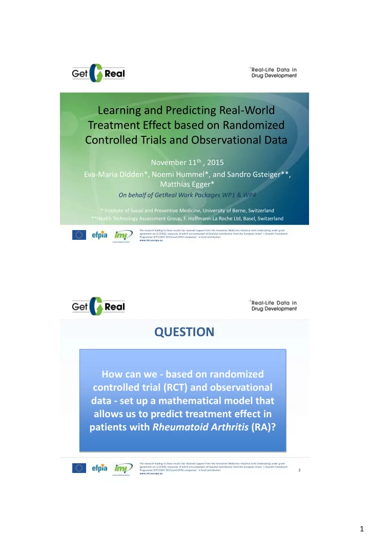
Learning and Predicting Real-World Treatment Effect based on Randomized Controlled Trials and Observational Data November 11 th , 2015 Eva-Maria Didden*, Noemi Hummel*, and Sandro Gsteiger**, Matthias Egger* On behalf of GetReal Work Packages WP1 & WP4 * Institute of Social and Preventive Medicine, University of Berne, Switzerland **Health Technology Assessment Group, F. Hoffmann-La Roche Ltd, Basel, Switzerland The research leading to these results has received support from the Innovative Medicines Initiative Joint Undertaking under grant agreement no [115303], resources of which are composed of financial contribution from the European Union ’ s Seventh Framework Programme (FP7/2007-2013) and EFPIA companies ’ in kind contribution. www.imi.europa.eu QUESTION How can we - based on randomized controlled trial (RCT) and observational data - set up a mathematical model that allows us to predict treatment effect in patients with Rheumatoid Arthritis (RA)? The research leading to these results has received support from the Innovative Medicines Initiative Joint Undertaking under grant agreement no [115303], resources of which are composed of financial contribution from the European Union ’ s Seventh Framework Programme (FP7/2007-2013) and EFPIA companies ’ in kind contribution. 2 www.imi.europa.eu 1
MODELLING PROCEDURE 1. Selection of a simple linear regression model for data from randomized controlled trials 2. Development of a marginal structural model (MSM) for observational data, to adjust for potential confounders 3. Incorporation of insights from both modelling approaches into a Bayesian inference framework 4. Prediction of treatment effect for a new real-world population, possibly under new study conditions The research leading to these results has received support from the Innovative Medicines Initiative Joint Undertaking under grant agreement no [115303], resources of which are composed of financial contribution from the European Union ’ s Seventh Framework Programme (FP7/2007-2013) and EFPIA companies ’ in kind contribution. 3 www.imi.europa.eu GRAPHICAL MODEL REPRESENTATION • Acyclic graph visualizing RCT conditions Covariates ( X ) Outcome ( Y ) Treatment ( Trt ) X • Acyclic graph visualizing real-world conditions V C Covariates ( C ) B Confounders Covariates ( B ) Outcome ( Y ) Treatment ( Trt ) Covariates ( V ) Non-Confounders The research leading to these results has received support from the Innovative Medicines Initiative Joint Undertaking under grant agreement no [115303], resources of which are composed of financial contribution from the European Union ’ s Seventh Framework Programme (FP7/2007-2013) and EFPIA companies ’ in kind contribution. 4 www.imi.europa.eu 2
VARIABLE SELECTION Outcome: RCT DATA OBSERVATIONAL DATA Change in Covariates X Covariates B Covariates V Confounders C E x DAS28 gender calendar year gender age p HAQ seropositivity hospital (y/n) baseline HAQ-DI disease duration e EQ5D baseline DAS28 Socio-economics steroid intake seropositivity r ACR baseline HAQ-DI …… # [concomitant smoking t DMARDs] (RA) CDAI # [previous anti- type of concomitant # [previous anti- TNF agents] DMARDs TNF agents] Stats RADAI ….. baseline DAS28 Confounders ( C ) comorbidities Covariates ( B ) Treatment Outcome ( Y ) # [previous Not DMARDs] Selec- Covariates ( V ) ted ….. The research leading to these results has received support from the Innovative Medicines Initiative Joint Undertaking under grant agreement no [115303], resources of which are composed of financial contribution from the European Union ’ s Seventh Framework Programme (FP7/2007-2013) and EFPIA companies ’ in kind contribution. 5 www.imi.europa.eu FORMAL MODEL REPRESENTATION 𝛽 : Intercept, 𝛾: Treatment effect • Linear model (LM) for RCT data: 𝛿 : (non-confounding) Covariate effect 2 𝐽 ) Y rct ~ 𝑂( 𝛽 𝑠𝑑𝑢 + 𝛾 𝑠𝑑𝑢 𝑈𝑠𝑢 + 𝛿 𝑠𝑑𝑢 𝑌 𝑠𝑑𝑢 , 𝜏 𝑠𝑑𝑢 𝑈𝑠𝑢 = 1, biological agent • MSM for the observational data: control treatment 0, weighted linear regression model 1 2 𝑋 −1 ) , 𝑋 Y 𝑝𝑐 ~ 𝑂( 𝛽 𝑝𝑐 + 𝛾 𝑝𝑐 𝑈𝑠𝑢 + 𝛿 𝑝𝑐 𝑊 𝑝𝑐 , 𝜏 𝑝𝑐 𝑝𝑐 ∝ 𝑔(𝑈𝑠𝑢|𝐷 𝑝𝑐 ) 𝑝𝑐 «If both models are sufficiently well specified and further MSM assumptions hold, the estimated treatment effects should be similar.» The research leading to these results has received support from the Innovative Medicines Initiative Joint Undertaking under grant agreement no [115303], resources of which are composed of financial contribution from the European Union ’ s Seventh Framework Programme (FP7/2007-2013) and EFPIA companies ’ in kind contribution. 6 www.imi.europa.eu 3
BAYESIAN MSM (BMSM) Likelihood: Gaussian MSM of the form 𝑍|Θ ~ 𝑂 𝛽 + 𝛾𝑈𝑠𝑢 + 𝛿𝑊, 𝜏 2 𝑋 −1 ; Θ = {𝛽, 𝛾, 𝛿, 𝜏 2 , Θ 𝑋 } Priors: 𝑠𝑑𝑢 , 𝜐 2 , where 𝜐 2 is based on expert opinions Set 𝛾 ~ 𝑂 𝛾 • • For the remaining parameters, choose suitable non- or weakly-informative priors Predictions: 1. Take the previously selected MSM structure and variables as a modelling basis 2. Estimate the posterior distributions of all unknown parameters 3. For any new set of observational data Y, draw posterior realizations (predictions) 1 , 𝑍 2 , … } from the according posterior predictive distribution 𝑪𝑵𝑻𝑵 = {𝑍 𝒁 The research leading to these results has received support from the Innovative Medicines Initiative Joint Undertaking under grant agreement no [115303], resources of which are composed of financial contribution from the European Union ’ s Seventh Framework Programme (FP7/2007-2013) and EFPIA companies ’ in kind contribution. 7 www.imi.europa.eu RESULTS ⋅ − 𝑍 , derived Residuals 𝑍 𝑚𝑛 − 𝑍 , under simple LM assumptions A posterior realiziation of residuals 𝑍 from our BMSM Distribution of 2 , … 1 𝑁𝑇𝐹 𝑍 , 𝑁𝑇𝐹 𝑍 𝑁𝑇𝐹 𝑍 𝑚𝑛 = 2.52 𝑂 = 1 2 − 𝑍 𝑁𝑇𝐹 𝑍 𝑂 𝑍 𝑗=1 The research leading to these results has received support from the Innovative Medicines Initiative Joint Undertaking under grant agreement no [115303], resources of which are composed of financial contribution from the European Union ’ s Seventh Framework Programme (FP7/2007-2013) and EFPIA companies ’ in kind contribution. 8 www.imi.europa.eu 4
DISCUSSION • Why using an MSM to adjust for confounding? – Flexibly applicable to different types of outcome and treatment data – Easily extendable to settings with time-varying treatment and confounding Most critical assumption: assumption of no unmeasured confounding • Why working on a Bayesian inference and prediction framework? – Inclusion of prior knowledge, possibly gained from multiple data sources – Estimation of posterior and posterior predictive distributions, and derivation of all measures of interest (e.g. posterior modus/mean of the parameters …) – Relaxation of the missing data problem • Work in progress: Development of suitable «goodness-of-fit-and-prediction» statistics The research leading to these results has received support from the Innovative Medicines Initiative Joint Undertaking under grant agreement no [115303], resources of which are composed of financial contribution from the European Union ’ s Seventh Framework Programme (FP7/2007-2013) and EFPIA companies ’ in kind contribution. 9 www.imi.europa.eu REFERENCES • A. Gelman, J. B. Carlin, H. S. Stern, and D. B. Rubin, Bayesian data analysis, Volume 2, London: Chapman & Hall/CRC, 2014. • A. Gelman, and X.-L. Meng (eds.), Applied Bayesian modeling and causal inference from incomplete-data perspectives , John Wiley & Sons, 2004. • J. M. Robins, M. A. Hernan, and B. Brumback, "Marginal structural models and causal inference in epidemiology." Epidemiology, Volume 11, Issue 5: 550-560, 2000. The research leading to these results has received support from the Innovative Medicines Initiative Joint Undertaking under grant agreement no [115303], resources of which are composed of financial contribution from the European Union ’ s Seventh Framework Programme (FP7/2007-2013) and EFPIA companies ’ in kind contribution. 10 www.imi.europa.eu 5
Recommend
More recommend