Quantum Time-Space Tradeoffs by Recording Queries Yassine Hamoudi, - PowerPoint PPT Presentation
Quantum Time-Space Tradeoffs by Recording Queries Yassine Hamoudi, Frdric Magniez IRIF , Universit de Paris arXiv: 2002.08944 Google Sycamores calculation Time 5 minutes Memory 53 qubits + few megabytes Simulation by
Finding 1 collision pair 23 Birthday attack + BHT algorithm Floyd’s cycle finding vs T = O ( N ) T = O ( N 1/3 ) S = O ( N 1/3 ) S = O (log N ) The quantum BHT algorithm has a better time complexity, but a worst time-space tradeo ff ! A BHT attack on SHA3-256 would require S ≈ 2 256/3 ≈ 2 85 qubits! Big open problem: Is there a quantum algorithm with and ? T ≤ o ( N ) S = O (log N )
Finding K collision pairs 24 Classical Tradeo ff Quantum Tradeo ff T 2 S ≤ Õ(K 2 N) T 2 S ≤ Õ(K 2 N) when when ̃ (log N) ≤ S ≤ Õ(K) ̃ (log N) ≤ S ≤ Õ(K 2/3 N 1/3 ) Ω Ω Upper bound Parallel Collision Search Adaptation of the BHT algorithm [van Oorschot and Wiener’99] ̃ (K 3 N) ̃ (K 2 N) T 2 S ≥ Ω T 3 S ≥ Ω Lower bound Our result [Dinur’20]
Finding K collision pairs 24 Classical Tradeo ff Quantum Tradeo ff T 2 S ≤ Õ(K 2 N) T 2 S ≤ Õ(K 2 N) when when ̃ (log N) ≤ S ≤ Õ(K) ̃ (log N) ≤ S ≤ Õ(K 2/3 N 1/3 ) Ω Ω Upper bound Parallel Collision Search Adaptation of the BHT algorithm [van Oorschot and Wiener’99] ̃ (K 3 N) ̃ (K 2 N) T 2 S ≥ Ω T 3 S ≥ Ω Lower bound Our result [Dinur’20]
Finding K collision pairs 24 Classical Tradeo ff Quantum Tradeo ff T 2 S ≤ Õ(K 2 N) T 2 S ≤ Õ(K 2 N) when when ̃ (log N) ≤ S ≤ Õ(K) ̃ (log N) ≤ S ≤ Õ(K 2/3 N 1/3 ) Ω Ω Upper bound Parallel Collision Search Adaptation of the BHT algorithm [van Oorschot and Wiener’99] ̃ (K 3 N) ̃ (K 2 N) T 2 S ≥ Ω T 3 S ≥ Ω Lower bound Our result [Dinur’20]
Finding K collision pairs 24 Classical Tradeo ff Quantum Tradeo ff T 2 S ≤ Õ(K 2 N) T 2 S ≤ Õ(K 2 N) when when ̃ (log N) ≤ S ≤ Õ(K) ̃ (log N) ≤ S ≤ Õ(K 2/3 N 1/3 ) Ω Ω Upper bound Parallel Collision Search Adaptation of the BHT algorithm [van Oorschot and Wiener’99] ̃ (K 3 N) ̃ (K 2 N) T 2 S ≥ Ω T 3 S ≥ Ω Lower bound Our result [Dinur’20] ̃ (K 2 N) We conjecture: T 2 S ≥ Ω
Finding K collision pairs 25 ̃ (K 3 N) Conjecture: T 2 S ≥ Ω ̃ (K 2 N) Our result: T 3 S ≥ Ω
Finding K collision pairs 25 ̃ (K 3 N) Conjecture: T 2 S ≥ Ω ̃ (K 2 N) Our result: T 3 S ≥ Ω • Our result is non-trivial when K ≥ ω (1):
Finding K collision pairs 25 ̃ (K 3 N) Conjecture: T 2 S ≥ Ω ̃ (K 2 N) Our result: T 3 S ≥ Ω • Our result is non-trivial when K ≥ ω (1): ̃ (N 1/3 ), which is the same as the time- → For K = 1 and S = log(N) it gives T ≥ Ω only lower bound [Aaronson and Shi’04].
Finding K collision pairs 25 ̃ (K 3 N) Conjecture: T 2 S ≥ Ω ̃ (K 2 N) Our result: T 3 S ≥ Ω • Our result is non-trivial when K ≥ ω (1): ̃ (N 1/3 ), which is the same as the time- → For K = 1 and S = log(N) it gives T ≥ Ω only lower bound [Aaronson and Shi’04]. ̃ (KN 1/3 ), whereas we prove that the → For K ≥ ω (1) and S = log(N) it gives T ≥ Ω ̃ (K 2/3 N 1/3 ). best time-only lower bound is T = Θ
Finding K collision pairs 25 ̃ (K 3 N) Conjecture: T 2 S ≥ Ω ̃ (K 2 N) Our result: T 3 S ≥ Ω • Our result is non-trivial when K ≥ ω (1): ̃ (N 1/3 ), which is the same as the time- → For K = 1 and S = log(N) it gives T ≥ Ω only lower bound [Aaronson and Shi’04]. ̃ (KN 1/3 ), whereas we prove that the → For K ≥ ω (1) and S = log(N) it gives T ≥ Ω ̃ (K 2/3 N 1/3 ). best time-only lower bound is T = Θ • The conjecture T 2 S ≥ Ω ̃ (N 3 ) for K = Θ ̃ (N) is particularly interesting:
Finding K collision pairs 25 ̃ (K 3 N) Conjecture: T 2 S ≥ Ω ̃ (K 2 N) Our result: T 3 S ≥ Ω • Our result is non-trivial when K ≥ ω (1): ̃ (N 1/3 ), which is the same as the time- → For K = 1 and S = log(N) it gives T ≥ Ω only lower bound [Aaronson and Shi’04]. ̃ (KN 1/3 ), whereas we prove that the → For K ≥ ω (1) and S = log(N) it gives T ≥ Ω ̃ (K 2/3 N 1/3 ). best time-only lower bound is T = Θ • The conjecture T 2 S ≥ Ω ̃ (N 3 ) for K = Θ ̃ (N) is particularly interesting: → Time-space tradeo ff s are generally easier to prove when the output is large.
Finding K collision pairs 25 ̃ (K 3 N) Conjecture: T 2 S ≥ Ω ̃ (K 2 N) Our result: T 3 S ≥ Ω • Our result is non-trivial when K ≥ ω (1): ̃ (N 1/3 ), which is the same as the time- → For K = 1 and S = log(N) it gives T ≥ Ω only lower bound [Aaronson and Shi’04]. ̃ (KN 1/3 ), whereas we prove that the → For K ≥ ω (1) and S = log(N) it gives T ≥ Ω ̃ (K 2/3 N 1/3 ). best time-only lower bound is T = Θ • The conjecture T 2 S ≥ Ω ̃ (N 3 ) for K = Θ ̃ (N) is particularly interesting: → Time-space tradeo ff s are generally easier to prove when the output is large. ̃ (N 2 ) for Element Distinctness. → If true, we show that it would implies T 2 S ≥ Ω
3 Lower Bounds by Recording Queries
Time-Space Lower Bounds from Time Lower Bounds 27 [Borodin et al.’81] : a general method to convert Time-only lower bounds directly into Time-Space lower bounds.
Time-Space Lower Bounds from Time Lower Bounds 27 [Borodin et al.’81] : a general method to convert Time-only lower bounds directly into Time-Space lower bounds. → The problem must have a large output ( ≠ decision problem). → The time lower bound is in the exponentially small success probability regime.
Time-Space Lower Bounds from Time Lower Bounds 27 [Borodin et al.’81] : a general method to convert Time-only lower bounds directly into Time-Space lower bounds. → The problem must have a large output ( ≠ decision problem). → The time lower bound is in the exponentially small success probability regime. [Klauck et al.’07, Ambainis’10, …] K-Search Finding K ones in x ∈ {0,1} N , | x | = K All existing quantum ⇒ with success probability at least 2 -O(K) time-space tradeo ff s requires time T ≥ Ω ( NK ) .
Time-Space Lower Bounds from Time Lower Bounds 27 [Borodin et al.’81] : a general method to convert Time-only lower bounds directly into Time-Space lower bounds. → The problem must have a large output ( ≠ decision problem). → The time lower bound is in the exponentially small success probability regime. [Klauck et al.’07, Ambainis’10, …] K-Search Finding K ones in x ∈ {0,1} N , | x | = K All existing quantum ⇒ with success probability at least 2 -O(K) time-space tradeo ff s requires time T ≥ Ω ( NK ) . K Collisions Finding K collisions in x ∼ [ N ] N ⇒ T 3 S ≥ ˜ Ω ( K 3 N ) with success probability at least 2 -O(K) for K-Collision Pairs Finding requires time T ≥ Ω ( K 2/3 N 1/3 ) .
Time Lower Bounds 28 Two main methods for proving quantum query lower bounds:
Time Lower Bounds 28 Two main methods for proving quantum query lower bounds: Polynomial Method The acceptance probability of a T-query algorithm is a polynomial in x of degree at most 2T.
Time Lower Bounds 28 Two main methods for proving quantum query lower bounds: Polynomial Method Adversary Method Bound the progress W t = ∑ x , y w x , y ⟨ ψ t The acceptance probability of a T-query algorithm x | ψ t y ⟩ . is a polynomial in x of degree at most 2T. x Q | 0 ⟩ … | ψ T x ⟩ | 0 ⟩ ⋮ | 0 ⟩
Time Lower Bounds 28 Two main methods for proving quantum query lower bounds: Polynomial Method Adversary Method Bound the progress W t = ∑ x , y w x , y ⟨ ψ t The acceptance probability of a T-query algorithm x | ψ t y ⟩ . is a polynomial in x of degree at most 2T. x Q | 0 ⟩ … | ψ T x ⟩ | 0 ⟩ ⋮ | 0 ⟩ Both methods are often di ffi cult to use in practice: K-Search in [Klauck et al.’07] K-Search in [Ambainis’10] Coppersmith-Rivlin’s bound + Extremal Analysis of the eigenspaces of properties of Chebyshev polynomials. the Johnson Association Scheme.
Time Lower Bounds 28 Two main methods for proving quantum query lower bounds: Polynomial Method Adversary Method Bound the progress W t = ∑ x , y w x , y ⟨ ψ t The acceptance probability of a T-query algorithm x | ψ t y ⟩ . is a polynomial in x of degree at most 2T. x Q | 0 ⟩ … | ψ T x ⟩ | 0 ⟩ ⋮ | 0 ⟩ Both methods are often di ffi cult to use in practice: K-Search in [Klauck et al.’07] K-Search in [Ambainis’10] Coppersmith-Rivlin’s bound + Extremal Analysis of the eigenspaces of properties of Chebyshev polynomials. the Johnson Association Scheme. A simpler and more intuitive method?
Classical Lower Bound for K-Search 29 Input: x = ( x 1 , …, x N ) where x i = 1 with probability K/N.
Classical Lower Bound for K-Search 29 Input: x = ( x 1 , …, x N ) where x i = 1 with probability K/N. Strategy: sample each entry only when it is queried, and record its value.
Classical Lower Bound for K-Search 29 Input: x = ( x 1 , …, x N ) where x i = 1 with probability K/N. Strategy: sample each entry only when it is queried, and record its value. Algorithm Input x = ( ⊥ , ⊥ , ⊥ , ⊥ )
Classical Lower Bound for K-Search 29 Input: x = ( x 1 , …, x N ) where x i = 1 with probability K/N. Strategy: sample each entry only when it is queried, and record its value. Algorithm Input x = ( ⊥ , ⊥ , ⊥ , ⊥ ) x 2 ?
Classical Lower Bound for K-Search 29 Input: x = ( x 1 , …, x N ) where x i = 1 with probability K/N. Strategy: sample each entry only when it is queried, and record its value. Algorithm Input x = ( ⊥ , ⊥ , ⊥ , ⊥ ) x 2 ? x = ( ⊥ , 0 , ⊥ , ⊥ )
Classical Lower Bound for K-Search 29 Input: x = ( x 1 , …, x N ) where x i = 1 with probability K/N. Strategy: sample each entry only when it is queried, and record its value. Algorithm Input x = ( ⊥ , ⊥ , ⊥ , ⊥ ) x 2 ? x = ( ⊥ , 0 , ⊥ , ⊥ ) x 2 = 0
Classical Lower Bound for K-Search 29 Input: x = ( x 1 , …, x N ) where x i = 1 with probability K/N. Strategy: sample each entry only when it is queried, and record its value. Algorithm Input x = ( ⊥ , ⊥ , ⊥ , ⊥ ) x 2 ? x = ( ⊥ , 0 , ⊥ , ⊥ ) x 2 = 0 x 1 ?
Classical Lower Bound for K-Search 29 Input: x = ( x 1 , …, x N ) where x i = 1 with probability K/N. Strategy: sample each entry only when it is queried, and record its value. Algorithm Input x = ( ⊥ , ⊥ , ⊥ , ⊥ ) x 2 ? x = ( ⊥ , 0 , ⊥ , ⊥ ) x 2 = 0 x 1 ? x = ( 1 , 0 , ⊥ , ⊥ )
Classical Lower Bound for K-Search 29 Input: x = ( x 1 , …, x N ) where x i = 1 with probability K/N. Strategy: sample each entry only when it is queried, and record its value. Algorithm Input x = ( ⊥ , ⊥ , ⊥ , ⊥ ) x 2 ? x = ( ⊥ , 0 , ⊥ , ⊥ ) x 2 = 0 x 1 ? x = ( 1 , 0 , ⊥ , ⊥ ) x 1 = 1
Classical Lower Bound for K-Search 29 Input: x = ( x 1 , …, x N ) where x i = 1 with probability K/N. Strategy: sample each entry only when it is queried, and record its value. Algorithm Input x = ( ⊥ , ⊥ , ⊥ , ⊥ ) x 2 ? x = ( ⊥ , 0 , ⊥ , ⊥ ) x 2 = 0 x 1 ? x = ( 1 , 0 , ⊥ , ⊥ ) x 1 = 1 x 2 ? x = ( 1 , 0 , ⊥ , ⊥ ) x 2 = 0 ⋮
Classical Lower Bound for K-Search 29 Input: x = ( x 1 , …, x N ) where x i = 1 with probability K/N. Strategy: sample each entry only when it is queried, and record its value. Algorithm Input x = ( ⊥ , ⊥ , ⊥ , ⊥ ) x 2 ? x = ( ⊥ , 0 , ⊥ , ⊥ ) x 2 = 0 x 1 ? x = ( 1 , 0 , ⊥ , ⊥ ) x 1 = 1 x 2 ? x = ( 1 , 0 , ⊥ , ⊥ ) x 2 = 0 ⋮ ≤ ( K /2 K /2 )( N ) T K Probability to have recorded at least K/2 ones after T queries
Classical Lower Bound for K-Search 29 Input: x = ( x 1 , …, x N ) where x i = 1 with probability K/N. Strategy: sample each entry only when it is queried, and record its value. Algorithm Input x = ( ⊥ , ⊥ , ⊥ , ⊥ ) x 2 ? x = ( ⊥ , 0 , ⊥ , ⊥ ) x 2 = 0 x 1 ? x = ( 1 , 0 , ⊥ , ⊥ ) x 1 = 1 x 2 ? x = ( 1 , 0 , ⊥ , ⊥ ) x 2 = 0 ⋮ ≤ ( K /2 K /2 )( N ) T K Probability to have recorded at least K/2 ones after T queries when T ≤ O ( N ) ≤ 2 −Ω ( K )
Classical Lower Bound for K-Search 29 Input: x = ( x 1 , …, x N ) where x i = 1 with probability K/N. Strategy: sample each entry only when it is queried, and record its value. Algorithm Input x = ( ⊥ , ⊥ , ⊥ , ⊥ ) x 2 ? x = ( ⊥ , 0 , ⊥ , ⊥ ) x 2 = 0 x 1 ? x = ( 1 , 0 , ⊥ , ⊥ ) x 1 = 1 x 2 ? x = ( 1 , 0 , ⊥ , ⊥ ) x 2 = 0 ⋮ ≤ ( K /2 K /2 )( N ) T K Probability to have recorded at least K/2 ones after T queries when T ≤ O ( N ) ≤ 2 −Ω ( K ) ≤ ( K / N ) K /2 ≤ 2 −Ω ( K ) (The un-recorded positions can only be guessed , with success ).
Recording of Quantum Queries 30 Can we record quantum queries similarly?
Recording of Quantum Queries 30 Can we record quantum queries similarly? [Zhandry’19]: • A quantum “recording technique” that works when the input x 1 , …, x N is sampled from the uniform distribution on [M] N . • Motivations: security proofs in the quantum random oracle model.
Recording of Quantum Queries 30 Can we record quantum queries similarly? [Zhandry’19]: • A quantum “recording technique” that works when the input x 1 , …, x N is sampled from the uniform distribution on [M] N . • Motivations: security proofs in the quantum random oracle model. Our contribution: • We generalize Zhandry’s technique to the case where x 1 , …, x N is sampled from any product distribution D 1 ⊗ … ⊗ D N on [M] N . • We simplify the framework and the analysis of the method.
Quantum Recording for K-Search 31 x 1 : 1 − K / N | 0 ⟩ + K / N | 1 ⟩ x 2 : 1 − K / N | 0 ⟩ + K / N | 1 ⟩ ⋮ x N : 1 − K / N | 0 ⟩ + K / N | 1 ⟩ Q Q Q | 0 ⟩ … | 0 ⟩ ⋮ | 0 ⟩ Query Operator x i ( − 1) x i | i ⟩ | i ⟩ Q
Quantum Recording for K-Search 32 x 1 : | ⊥ ⟩ x 2 : | ⊥ ⟩ ? ? ? R R R ⋮ x N : | ⊥ ⟩ | 0 ⟩ … | 0 ⟩ ⋮ | 0 ⟩ Query Operator x i ( − 1) x i | i ⟩ | i ⟩ Q
Quantum Recording for K-Search 32 x 1 : | ⊥ ⟩ x 2 : | ⊥ ⟩ ? ? ? R R R ⋮ x N : | ⊥ ⟩ | 0 ⟩ … | 0 ⟩ ⋮ | 0 ⟩ S | ⊥ ⟩ = 1 − K / N | 0 ⟩ + K / N | 1 ⟩ Query Operator x i ( − 1) x i | i ⟩ | i ⟩ Q
Quantum Recording for K-Search 32 x 1 : | ⊥ ⟩ S x 2 : | ⊥ ⟩ S R R R ⋮ x N : | ⊥ ⟩ S | 0 ⟩ … | 0 ⟩ ⋮ | 0 ⟩ S | ⊥ ⟩ = 1 − K / N | 0 ⟩ + K / N | 1 ⟩ Recording Query Operator Query Operator x i x i S † S ( − 1) x i | i ⟩ | i ⟩ Q | i ⟩ Q R ( − 1) ⊥ = 1 (where )
Quantum Recording for K-Search 32 x 1 : | ⊥ ⟩ S x 2 : | ⊥ ⟩ S R R R ⋮ x N : | ⊥ ⟩ S | 0 ⟩ … | 0 ⟩ ⋮ | 0 ⟩ S | ⊥ ⟩ = 1 − K / N | 0 ⟩ + K / N | 1 ⟩ Recording Query Operator Query Operator We show that it makes no x i x i S † di ff erence for the algorithm. S ( − 1) x i | i ⟩ | i ⟩ Q | i ⟩ Q R ( − 1) ⊥ = 1 (where )
Quantum Recording for K-Search 32 x 1 : | ⊥ ⟩ S x 2 : | ⊥ ⟩ S R R R ⋮ x N : | ⊥ ⟩ S | 0 ⟩ … | 0 ⟩ ⋮ | 0 ⟩ S | ⊥ ⟩ = 1 − K / N | 0 ⟩ + K / N | 1 ⟩ Recording Query Operator Query Operator We show that it makes no x i x i S † di ff erence for the algorithm. S We show that it “records” the 1’s. ( − 1) x i | i ⟩ | i ⟩ Q | i ⟩ Q R ( − 1) ⊥ = 1 (where )
Quantum Recording for K-Search 33 x 1 : 1 − K / N | 0 ⟩ + K / N | 1 ⟩ x 2 : 1 − K / N | 0 ⟩ + K / N | 1 ⟩ ⋮ x N : 1 − K / N | 0 ⟩ + K / N | 1 ⟩ Q Q Q | 0 ⟩ … | 0 ⟩ ⋮ | 0 ⟩ S | ⊥ ⟩ = 1 − K / N | 0 ⟩ + K / N | 1 ⟩
Quantum Recording for K-Search 33 x 1 : | ⊥ ⟩ S x 2 : | ⊥ ⟩ S ⋮ x N : | ⊥ ⟩ S Q Q Q | 0 ⟩ … | 0 ⟩ ⋮ | 0 ⟩ S | ⊥ ⟩ = 1 − K / N | 0 ⟩ + K / N | 1 ⟩
Quantum Recording for K-Search 33 x 1 : | ⊥ ⟩ S x 2 : | ⊥ ⟩ S ⋮ x N : | ⊥ ⟩ S Q Q Q | 0 ⟩ … | 0 ⟩ ⋮ | 0 ⟩ S | ⊥ ⟩ = 1 − K / N | 0 ⟩ + K / N | 1 ⟩
Quantum Recording for K-Search 33 x 1 : S † | ⊥ ⟩ S S x 2 : | ⊥ ⟩ S † S S ⋮ x N : | ⊥ ⟩ S † S S Q Q Q | 0 ⟩ … | 0 ⟩ ⋮ | 0 ⟩ S | ⊥ ⟩ = 1 − K / N | 0 ⟩ + K / N | 1 ⟩
Quantum Recording for K-Search 33 x 1 : S † S † | ⊥ ⟩ S S x 2 : | ⊥ ⟩ S † S † S S ⋮ x N : S † | ⊥ ⟩ S † S S Q Q Q | 0 ⟩ … | 0 ⟩ ⋮ | 0 ⟩ S | ⊥ ⟩ = 1 − K / N | 0 ⟩ + K / N | 1 ⟩
Quantum Recording for K-Search 33 x 1 : S † S † | ⊥ ⟩ S S S x 2 : | ⊥ ⟩ S † S † S S S ⋮ x N : S † | ⊥ ⟩ S † S S S Q Q Q | 0 ⟩ … | 0 ⟩ ⋮ | 0 ⟩ S | ⊥ ⟩ = 1 − K / N | 0 ⟩ + K / N | 1 ⟩
Quantum Recording for K-Search 33 x 1 : S † S † | ⊥ ⟩ S † S S S S x 2 : | ⊥ ⟩ S † S † S † S S S S ⋮ x N : S † | ⊥ ⟩ S † S † S S S S Q Q Q | 0 ⟩ … | 0 ⟩ ⋮ | 0 ⟩ S | ⊥ ⟩ = 1 − K / N | 0 ⟩ + K / N | 1 ⟩
Quantum Recording for K-Search 33 x 1 : S † S † | ⊥ ⟩ S † S S S S x 2 : | ⊥ ⟩ S † S † S † S S S S ⋮ x N : S † | ⊥ ⟩ S † S † S S S S Q Q Q | 0 ⟩ … | 0 ⟩ ⋮ | 0 ⟩ S | ⊥ ⟩ = 1 − K / N | 0 ⟩ + K / N | 1 ⟩ Recording Query Operator S † x 1 S ⋮ x i S † S ⋮ x N S † S Q | i ⟩ R
Quantum Recording for K-Search 33 x 1 : S † S † | ⊥ ⟩ S † S S S S x 2 : | ⊥ ⟩ S † S † S † S S S S ⋮ x N : S † | ⊥ ⟩ S † S † S S S S Q Q Q | 0 ⟩ … | 0 ⟩ ⋮ | 0 ⟩ S | ⊥ ⟩ = 1 − K / N | 0 ⟩ + K / N | 1 ⟩ Recording Query Operator If x j is not queried it stays unchanged. x i S † S Q | i ⟩ R
Quantum Recording for K-Search 33 x 1 : | ⊥ ⟩ S x 2 : | ⊥ ⟩ S R R R ⋮ x N : | ⊥ ⟩ S | 0 ⟩ … | 0 ⟩ ⋮ | 0 ⟩ S | ⊥ ⟩ = 1 − K / N | 0 ⟩ + K / N | 1 ⟩ Recording Query Operator If x j is not queried it stays unchanged. x i S † S Q | i ⟩ R
Quantum Recording for K-Search 33 x 1 : | ⊥ ⟩ S x 2 : | ⊥ ⟩ S R R R ⋮ x N : | ⊥ ⟩ S | 0 ⟩ … | 0 ⟩ ⋮ | 0 ⟩ S | ⊥ ⟩ = 1 − K / N | 0 ⟩ + K / N | 1 ⟩ | ⊥ ⟩ R Recording Query Operator | i ⟩ | 0 ⟩ x i S † R S | i ⟩ Q | i ⟩ | 1 ⟩ R R | i ⟩
Quantum Recording for K-Search 33 x 1 : | ⊥ ⟩ S x 2 : | ⊥ ⟩ S R R R ⋮ x N : | ⊥ ⟩ S | 0 ⟩ … | 0 ⟩ ⋮ | 0 ⟩ S | ⊥ ⟩ = 1 − K / N | 0 ⟩ + K / N | 1 ⟩ | ⊥ ⟩ ≈ | ⊥ ⟩ − K / N | 1 ⟩ R Recording Query Operator | i ⟩ | i ⟩ | 0 ⟩ x i S † R S | i ⟩ Q | i ⟩ | 1 ⟩ R R | i ⟩
Quantum Recording for K-Search 33 x 1 : | ⊥ ⟩ S x 2 : | ⊥ ⟩ S R R R ⋮ x N : | ⊥ ⟩ S | 0 ⟩ … | 0 ⟩ ⋮ | 0 ⟩ S | ⊥ ⟩ = 1 − K / N | 0 ⟩ + K / N | 1 ⟩ | ⊥ ⟩ ≈ | ⊥ ⟩ − K / N | 1 ⟩ R Recording Query Operator | i ⟩ | i ⟩ | 0 ⟩ ≈ | 0 ⟩ + K / N | 1 ⟩ x i S † R S | i ⟩ | i ⟩ Q | i ⟩ | 1 ⟩ R R | i ⟩
Quantum Recording for K-Search 33 x 1 : | ⊥ ⟩ S x 2 : | ⊥ ⟩ S R R R ⋮ x N : | ⊥ ⟩ S | 0 ⟩ … | 0 ⟩ ⋮ | 0 ⟩ S | ⊥ ⟩ = 1 − K / N | 0 ⟩ + K / N | 1 ⟩ | ⊥ ⟩ ≈ | ⊥ ⟩ − K / N | 1 ⟩ R Recording Query Operator | i ⟩ | i ⟩ | 0 ⟩ ≈ | 0 ⟩ + K / N | 1 ⟩ x i S † R S | i ⟩ | i ⟩ Q | i ⟩ K / N ( | 0 ⟩ − | ⊥ ⟩ ) | 1 ⟩ ≈ − | 1 ⟩ + R R | i ⟩ | i ⟩
Quantum Recording for K-Search 33 x 1 : | ⊥ ⟩ S x 2 : | ⊥ ⟩ S R R R ⋮ x N : | ⊥ ⟩ S | 0 ⟩ … | 0 ⟩ ⋮ | 0 ⟩ S | ⊥ ⟩ = 1 − K / N | 0 ⟩ + K / N | 1 ⟩ | ⊥ ⟩ ≈ | ⊥ ⟩ − K / N | 1 ⟩ R Recording Query Operator Record | i ⟩ | i ⟩ a new 1 | 0 ⟩ ≈ | 0 ⟩ + K / N | 1 ⟩ x i S † R S | i ⟩ | i ⟩ Q | i ⟩ K / N ( | 0 ⟩ − | ⊥ ⟩ ) | 1 ⟩ ≈ − | 1 ⟩ + R R | i ⟩ | i ⟩
Quantum Recording 34 Classical Recording Quantum Recording Probability to have recorded Amplitude of the states that have at least K/2 ones recorded at least K/2 ones K-Search ≤ ( ≤ ( K /2 K /2 K /2 )( N ) K /2 )( 4 N ) T K T K Probability to have recorded Amplitude of the states that have at least K/2 (disjoint) collisions recorded at least K/2 (disjoint) collisions K-Collision Pairs ≤ ( ≤ ( K /2 K /2 K /2 )( N ) K /2 )( 4 N ) T T T T
Recommend


More recommend
Explore More Topics
Stay informed with curated content and fresh updates.