Q-learning 3-23-16 Markov Decision Processes (MDPs) States: S - PowerPoint PPT Presentation
Q-learning 3-23-16 Markov Decision Processes (MDPs) States: S Actions A vs. A s Transition probabilities: P(s | s, a) Rewards R(s) vs. R(s,a) vs. R(s,s) Discount factor (sometimes considered part of the
Q-learning 3-23-16
Markov Decision Processes (MDPs) ● States: S ● Actions ○ A vs. A s ● Transition probabilities: P(s’ | s, a) ● Rewards ○ R(s) vs. R(s,a) vs. R(s,s’) ● Discount factor (sometimes considered part of the environment, sometimes part of the agent).
Reward vs. Value ● Reward is how the agent receives feedback in the moment. ● The agent wants to maximize reward over the long term. ● Value is the reward the agent expects in the future. ○ Expected sum of discounted future reward. � = discount r t = reward at time t
Why do we use discounting? We want the agent to act over infinite horizons. ● Without discounting, the sum of rewards would be infinite. ● With discounting, as long as rewards are bounded, the sum converges. We also want the agent to accomplish its goals quickly when possible. ● Discounting causes the agent to prefer receiving rewards sooner.
Known vs. unknown MDPs If we know the full MDP: ● All states and actions ● All transition probabilities ● All rewards Then we can use value iteration to find an optimal policy before we start acting. If we don’t know the full MDP: ● Missing states (we generally assume we know actions) ● Missing transition probabilities ● Missing rewards Then we need to try out various actions to see what happens. This is RL.
Temporal difference (TD) learning Key idea: Use the differences in utilities between successive states Update rule: Equivalently: � = learning rate � = discount temporal difference s ′ = next state
How the heck does TD learning work? TD learning maintains no model of the environment. ● It never learns transition probabilities. Yet TD learning converges to correct value estimates. Why? Consider how values will be modified... ● when all values are initially 0. ● when future value is higher than current. ● when future value is lower than current. ● when discount is close to 1. ● when discount is close to 0.
Q-learning Key idea: temporal difference learning on (state, action) pairs. ● Q(s,a) denotes the expected value of doing action a in state s. ● Store Q values in a table, and update them incrementally. Update rule: Equivalently:
Exercise: carry out Q-learning discount: 0.9 learning rate: 0.2 0 0 0 We’ve already seen the terminal states. +1 0 0 0 0 0 0 2 Use these exploration traces: 0 0 0 (0,0)→(1,0)→(2,0)→(2,1)→(3,1) 0 0 -1 0 0 0 0 1 (0,0)→(0,1)→(0,2)→(1,2)→(2,2)→(3,2) 0 0 (0,0)→(0,1)→(0,2)→(1,2)→(2,2)→(2,1)→(3,1) 0 0 0 0 0 0 0 0 0 0 0 0 (0,0)→(1,0)→(2,0)→(2,1)→(2,2)→(3,2) 0 0 0 0 0 (0,0)→(1,0)→(2,0)→(3,0)→(3,1) 0 1 2 3 (0,0)→(0,1)→(0,2)→(1,2)→(2,2)→(3,2)
Exploration policy vs. optimal policy Where do the exploration traces come from? ● We need some policy for acting in the environment before we understand it. ● We’d like to get decent rewards while exploring. ○ Explore/exploit tradeoff. In lab, we’re using an epsilon-greedy exploration policy. After exploration, taking random bad moves doesn’t make much sense. ● If Q-value estimates are correct a greedy policy is optimal.
Recommend
More recommend
Explore More Topics
Stay informed with curated content and fresh updates.
