Prof Emmanuel Agu Computer Science Dept. Worcester Polytechnic - PowerPoint PPT Presentation
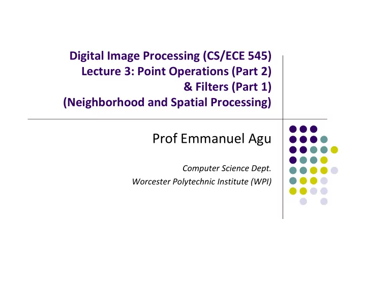
Digital Image Processing (CS/ECE 545) Lecture 3: Point Operations (Part 2) & Filters (Part 1) (Neighborhood and Spatial Processing) Prof Emmanuel Agu Computer Science Dept. Worcester Polytechnic Institute (WPI) Recall: Histogram Equalization
Digital Image Processing (CS/ECE 545) Lecture 3: Point Operations (Part 2) & Filters (Part 1) (Neighborhood and Spatial Processing) Prof Emmanuel Agu Computer Science Dept. Worcester Polytechnic Institute (WPI)
Recall: Histogram Equalization Adjust 2 different images to make their histograms (intensity distributions) similar Apply a point operation that changes histogram of modified image into uniform distribution Histogram Cumulative Histogram
Images taken from Gonzalez & Woods, Digital Image Processing (2002) Function Recall: Equalization Transformation
Linear Histogram Equalization Histogram cannot be made exactly flat – peaks cannot be increased or decreased by point operations. Following point operation makes histogram as flat as possible: (assuming M x N image and pixels in range [0, K ‐ 1]) Point operation that returns Linear equalized value of a Cumulative Histogram: Σ how many times intensity a occurs
Effects of Linear Histogram Equalization Original Image I Image I’ after Linear Equalization Original Histogram after histogram Linear Equalization Cumulative Histogram Cumulative After Linear Histogram Equalization
Sample Linear Equalization Code Obtain histogram of image ip Compute cumulative histogram in place Get intensity value at (u,v) Equalize pixel intensity Cumulative Histogram: Σ how many times intensity a occurs
Histogram Specification Real images never show uniform distribution (unnatural) Most real images, distribution of pixel intensities is gaussian Histogram specification modifies an image’s histogram into an arbitrary intensity distribution (may not be uniform) Image 1’s histogram can also be used as target for image 2 Why? Makes images taken by 2 different cameras to appear as if taken by same camera
Images and Probability
Histogram Specification Find a mapping such that distribution of a matches some reference distribution.i.e Mapping function: maps distribution on right to equivalent point (same height) On distribution on left to convert original image I A into I A’ such that i.e. a and a’ have same height (b) on different CDF distributions P A (a) P -1 R (b)
Adjusting Linear Distribution Piecewise In practice, reference distribution may be specified as a piecewise linear function 2 endpoints are fixed
Adjusting Linear Distribution Piecewise For each segment, linearly Interpolate to find any value We also need the inverse mapping
Adjusting Linear Distribution Piecewise
Adjusting Linear Histogram Piecewise
Histogram Matching Prior method needed reference distribution to be invertible Has to be invertible What if reference histogram is not invertible? For example not invertible if histogram has some intensities that occur with probability 0? i.e. p(k) = 0 Use different method called histogram matching
Histogram Matching
Adjusting to a Given Histogram Reference Height of original Cumulative Intensity on Distribution histogram Matched intensity Original intensity
Adjusting to a Given Histogram
Adjusting to a Given Histogram Original histogram after matching original histogram CDF of original CDF of original histogram after histogram matching
Adjusting to a Given Histogram
Gamma Correction Camera Electric Light Signal Light Electric Signal Display Different camera sensors Have different responses to light intensity Produce different electrical signals for same input How do we ensure there is consistency in: Images recorded by different cameras for given light input a) Light emitted by different display devices for same image? b)
Gamma Correction What is the relation between: Camera: Light on sensor vs. “intensity” of corresponding pixel Display: Pixel intensity vs. light from that pixel Relation between pixel value and corresponding physical quantity is usually complex, nonlinear An approximation ?
What is Gamma? Originates from analog photography Exposure function: relationship between: logarithmic light intensity vs. resulting film density. Film density Gamma: slope of linear (measure of response) range of the curve The same in TV broadcasting Log of light intensity
What is Gamma? Gamma function: a good approximation of exposure curve Inverse of a Gamma function is another gamma function with Gamma of CRT and LCD monitors: 1.8 ‐ 2.8 (typically 2.4) Output signal Raised by gamma Correct output signal By dividing by 1/ gamma (called Gamma correction)
Gamma Correction Obtain a measurement b proportional to original light intensity B by applying inverse gamma function Gamma correction is important to achieve a device independent representation
Gamma Correction
Gamma Correction Code Compute corrected intensity and store in lookup table fgc
Point Operations in ImageJ
ImageJ Operations involving 2 images
Example: Alpha Blending
Alpha Blending PlugIn
What Is Image Enhancement? Image enhancement makes images more useful by: Highlighting interesting detail in images Removing noise from images Making images more visually appealing
Images taken from Gonzalez & Woods, Digital Image Processing (2002) Image Enhancement Examples
Images taken from Gonzalez & Woods, Digital Image Processing (2002) Image Enhancement Examples (cont…)
Images taken from Gonzalez & Woods, Digital Image Processing (2002) Image Enhancement Examples (cont…)
Images taken from Gonzalez & Woods, Digital Image Processing (2002) Image Enhancement Examples (cont…)
Spatial & Frequency Domains There are two broad categories of image enhancement techniques Spatial domain techniques Direct manipulation of image pixels (intensity values) Frequency domain techniques Manipulation of Fourier transform or wavelet transform of an image First spatial domain techniques Later: frequency domain techniques
What is a Filter? Capabilities of point operations are limited Filters: combine pixel’s value + values of neighbors E.g blurring: Compute average intensity of block of pixels Combining multiple pixels needed for certain operations: Blurring, Smoothing Sharpening
What Point Operations Can’t Do Example: sharpening
What Point Operations Can’t Do Other cool artistic patterns by combining pixels
Definition: Spatial Filter
Example: Average (Mean) of 3x3 Neighborhood pixel 8 neighbor pixel Blurring: Replace each pixel with AVERAGE Intensity of pixel + neighbors
Smoothing an Image by Averaging Replace each pixel by average of pixel + neighbors For 3x3 neighborhood:
Smoothing an Image by Averaging
Example: Smoothing Spatial Filtering Origin x 1 / 9 1 / 9 1 / 9 104 100 108 1 / 9 1 / 9 1 / 9 * 99 106 98 1 / 9 1 / 9 1 / 9 95 90 85 Original Image Filter 1 / 9 1 / 9 1 / 9 104 100 108 Simple 3*3 3*3 Smoothing Pixels 1 / 9 1 / 9 1 / 9 99 98 106 Neighbourhood Filter 1 / 9 1 / 9 1 / 9 95 90 85 e = 1 / 9 *106 + 1 / 9 *104 + 1 / 9 *100 + 1 / 9 *108 + 1 / 9 *99 + 1 / 9 *98 + 1 / 9 *95 + 1 / 9 *90 + 1 / 9 *85 y Image f (x, y) = 98.3333 The above is repeated for every pixel in the original image to generate the smoothed image
Smoothing an Image by Averaging Previous example: Filter size: 3x3 Many possible filter parameters (size, weights, function, etc) Filter size (size of neighborhood): 3x3, 5x5, 7x7, …,21x21,.. Filter shape: not necessarily square. Can be rectangle, circle, etc Filter weights: May apply unequal weighting to different pixels Filters function: can be linear (a weighted summation) or nonlinear
The Filter Matrix Filter operation can be expressed as a matrix Example: averaging filter Filter matrix also called filter mask H(i,j)
Example: What does this Filter Do?
What Does this Filter Do?
Mean Filters: Effect of Filter Size
Applying Linear Filters: Convolution 2. Multiply all filter coefficients H(i,j) For each image position I(u,v): with corresponding pixel I(u + i, v + j) 1. Move filter matrix H over image such that H(0,0) 3. Sum up results and store coincides with current image sum in corresponding position position (u,v) in new image I’(u, v) Stated formally: R H is set of all pixels Covered by filter. For 3x3 filter, this is:
Computing Filter Operation Filter matrix H moves over each pixel in original image I to compute corresponding pixel in new image I’ Cannot overwrite new pixel value in original image I Why? Copy original image I to intermediate Store results I’ in intermediate image, use it as source, then store image, then copy back to replace I results I’ to replace original image
Simple 3x3 Averaging Filter (“Box” Filter) No explicit filter matrix since all coefficients are the same (1/9) No clamping required Make copy of original image to use as source Loop over all pixels in image Filter computation by adding current pixel’s neighbors Store result back in original image
Recommend
More recommend
Explore More Topics
Stay informed with curated content and fresh updates.
