Probability/Statistics Review & Linear Regression Lecturer: Roni - PDF document
10-601A: Machine Learning, Spring 2015 Probability/Statistics Review & Linear Regression Lecturer: Roni Rosenfeld Scribe: Udbhav Prasad 1 Probability and Statistics A regular variable holds, at any one time, a single value, be it numeric or
10-601A: Machine Learning, Spring 2015 Probability/Statistics Review & Linear Regression Lecturer: Roni Rosenfeld Scribe: Udbhav Prasad 1 Probability and Statistics A regular variable holds, at any one time, a single value, be it numeric or otherwise. In contrast, a random variable (RV) holds a distribution over values, be they numeric or otherwise. For example, the outcome of a future toss of a fair coin can be captured by a random variable X holding the following distribution: ’HEAD’ with probability 0.5, and ’TAIL’ with probability 0.5 . We will use uppercase characters to denote random variables, and their lowercase equivalents to denote the values taken by those random variables. The following are commonly used notations to represent probabili- ties: 1. Pr( x ) is shorthand for Pr( X = x ) 2. Pr( x, y ) is shorthand for Pr( X = x AND Y = y ) 3. Pr( x | y ) is shorthand for Pr( X = x | Y = y ) In a multivariate distribution over X and Y , the marginal of X is � Pr X ( x ) = Pr( x, y ) y and the marginal of Y is � Pr Y ( y ) = Pr( x, y ) x The Chain Rule is: Pr( x, y ) = Pr( x | y ) Pr( y ) = Pr( y | x ) Pr( x ) Independence of two random variables X and Y is defined as follows ( ⊥ ⊥ is the symbol for independence): X ⊥ ⊥ Y ⇐ ⇒ ∀ x ∈ X, y ∈ Y, Pr( x, y ) = Pr( x ) Pr( y ) X ⊥ ⊥ Y ⇐ ⇒ Y ⊥ ⊥ X Expected value or mean of a RV is defined (for a discrete RV) as: � E[ X ] = x Pr( x ) x 1
2 Probability/Statistics Review & Linear Regression Properties of E: 1. E is a linear operator: E[ aX + b ] = a E[ X ] + b . 2. E[ aX + bY + c ] = a E[ X ] + b E[ Y ] + c (note that this doesn’t assume any relationship between X and Y ). 3. E[ � i f i ( X, Y, Z . . . )] = � i E[ f i ( X, Y, Z . . . )] where f i s are some functions of the random variables. Again, note that this does not assume anything about the f i s or the relationship among X, Y, Z . . . . 4. In general, E[ f ( X )] � = f (E[ X ]). For example, E[ X 2 ] is often not equal to (E[ X ]) 2 (incidentally (E[ X ]) 2 can also be denoted as E 2 [ X ]). In fact, for the specific case of f ( X ) = X 2 , it is always true that E[ f ( X )] ≥ f (E[ X ]). Variance Var[ X ] of a random variable X (also denoted as σ 2 ( X )) is defined as: Var[ X ] = E[( X − E[ X ]) 2 ] Variance is the second moment of the RV about its mean (also known as the second central moment). Its units are the square of the units of the original RV. A useful alternative formula for the variance: Var[ X ] = E[ X 2 ] − E 2 [ X ] � Standard deviation σ ( X ) of X is defined as: σ ( X ) = Var[ X ] The Covariance of X and Y , also written as σ ( X, Y ), is defined as: Cov[ X, Y ] = E[( X − E[ X ])( Y − E[ Y ])] = E[( XY − E[ X ] Y − X E[ Y ] + E[ X ]E[ Y ])] = E[ XY ] − (E[ X ])(E[ Y ]). So Cov[ X, Y ] = 0 ⇐ ⇒ E[ XY ] = (E X )(E Y ). Properties of Var, σ and Cov ( a , b and c are real constants): 1. Var[ X + b ] = Var[ X ]. 2. Var[ aX ] = a 2 Var[ X ]. 3. Var[ aX + b ] = a 2 Var[ X ]. 4. Var[ X + Y ] = Var[ X ] + Var[ Y ] + 2Cov[ X, Y ] 5. Var[ aX + bY + c ] = Var[ aX + bY ] = a 2 Var[ X ] + b 2 Var[ Y ] + 2 ab Cov[ X, Y ]. 6. Var[ � i w i X i ] = � i,j w i w j Cov[ X i , X j ]. (Note that Var[ X i ] = Cov[ X i , X i ]) 7. Variance of uncorrelated variables is additive: ( ∀ i, ∀ j � = i Cov[ Xi, Xj ] = 0) = ⇒ Var[ � i X i ] = � i Var[ X i ]. 8. Var[ X ] = Cov[ X, X ]. 9. σ ( aX + b ) = | a | ∗ σ ( X ). 10. Cov[ aX + b, cY + d ] = Cov[ aX, cY ] = ac Cov[ X, Y ]. Covariance is invariant under shift of either variable. The Law of Total Variance: Var[ Y ] = Var X [E[ Y | X ]] + E X [Var[ Y | X ]] In clustering, the first term is the cross-cluster variance , and the second term is the within-cluster variance . In regression, the first term is the explained variance , and the second term is the unexplained variance .
Probability/Statistics Review & Linear Regression 3 Linear Correlation , Corr[ X, Y ], often loosely called just ’correlation’, is defined as Corr[ X, Y ] = ρ ( X, Y ) = Cov[ X, Y ] ∈ [ − 1 , +1] σ ( X ) σ ( Y ) Correlation is invariant under shift and scale of either variable (up to change of sign): ρ ( aX + b, cY + d ) = sign ( ac ) ρ ( X, Y ) X ′ = ( X − E[ X ]) /σ ( X ) Y ′ = ( Y − E[ Y ]) /σ ( Y ) X’, Y’ are zero-mean, unit-variance = ⇒ ρ ( X, Y ) = ρ ( X ′ , Y ′ ) = E[ X ′ Y ′ ]. X ⊥ ⊥ Y = ⇒ ρ = 0, but not vice versa! X, Y can be (linearly) uncorrelated, but still dependent! (think of the case of distribution of points on the circumference of a circle). Linear correlation measures only the extent to which X, Y are linearly related and not some other relationship between them. Summary: Independent = ⇒ uncorrelated. 2 Correlation vs. Mutual Information Recall the definitions of Mutual Information Pr( x, y ) � � I( X ; Y ) = E log Pr( x ) Pr( y ) and Linear Correlation Corr[ X, Y ] = ρ ( X, Y ) = Cov[ X, Y ] σ ( X ) σ ( Y ) (Linear) Correlation requires the x, y values to be numerical, so that there is a notion of distance between two values — a metric space. It measures the extent or tightness of linear association, not its slope. Linear correlation is invariant under a linear transformation (shifting and scaling) of either variable on its own. Note however that correlation is not invariant to rotation, because rotation of the ( X, Y ) plane corresponds to a joint linear transformation of the two variables: the new X variable is a function of both the old X and the old Y , and similarly for the new Y variable. This allows the correlation to change. To calculate correlation between two binary RVs, treat each RV as having any two numerical values, say 0 and 1 — it doesn’t matter what two values are chosen. ρ is dimensionless – it is a pure number. Its range: ρ ∈ [ − 1 , +1]. Often we care only about the strength of the correlation, rather than its polarity. In that case we tend to look at ρ 2 which is in the range [0 , 1]. In fact, ρ 2 has an important interpretation: it is the fraction of the variance of Y that’s explained by X (compare to the Law of Total Variance above). In contrast, mutual information does not require a metric space. X and/or Y could take on any values, e.g. X = { blue, red, green } , Y = { math, physics } . Range: 0 ≤ I( X, Y ) ≤ min( H ( X ) , H ( Y )) Dimension: bits. ⇒ X ⊥ ⊥ Y . I( X ; Y ) = 0 ⇐ Examples of high mutual information (I( X ; Y )) but correlation ( ρ ) = 0 :
4 Probability/Statistics Review & Linear Regression 1. A perfect polygon, with uniform probability distribution on the vertices. ρ ( X, Y ) is always 0, but as the number of vertices goes to infinity, so does I( X ; Y ). 2. Smallest example: Uniform distribution on the vertices of an equilateral triangle. 3. Consider a uniform distribution over the vertices of a square, and consider what happens when you rotate the square. Correlation is preserved (at 0), because rotation corresponds to linear transformation of each random variable. But mutual information is not invariant to rotation! When the square is axis parallel, I ( X ; Y ) is reduced. ⇒ X ⊥ ⊥ Y = I( X ; Y ) = 0 ⇐ ⇒ ρ ( X, Y ) = 0 Can we have zero mutual information but non-zero correlation? No, because I( X ; Y ) = 0 means X, Y are independent, so ρ = 0. But we can have high correlation (1.0) with arbirarily low mutual information. For example, consider the 2x2 joint distribution: X \ Y 0 1 0 1 − ǫ 0.0 1 0.0 ǫ Interpretation: the degree of association between X,Y is very very high. In fact, one can perfectly fit a straight line, so ρ ( X, Y ) = 1. However, I ( X ; Y ) = H ( Y ) = H (1 − ǫ, ǫ ). As ǫ → 0, mutual information gets arbitrarily close to zero. 3 Linear Learning in One Dimension (Simple Linear Regression) Our goal is to learn a (not necessarily deterministic) mapping f : X → Y . Because the mapping is typically non-deterministic, we will view ( X, Y ) as jointly distributed according to some distribution p ( x, y ). Since X (the input) will be given to us, we are interested in learning p ( y | x ) rather than p ( x, y ). To simplify, we will focus on learning, given any x , the expected value of Y , namely, E[ Y | X = x ]. To simplify further, we will assume a linear relationship between X and E[ Y ]: E[ Y | X ] = α + βX Or, equivalently: Y = α + βX + ǫ where ǫ is some zero-mean distribution. This is called a linear model. α, β are the parameters of the model. β is the slope, α is the intercept, or offset. Given a set of data { X i , Y i } n i =1 , how should we estimate the parameters α, β ? For any given values of α, β , we can plot the line on top of the datapoints, and consider the ’errors’, or residuals : ǫ i = y i − ( α + βx i )
Recommend
More recommend
Explore More Topics
Stay informed with curated content and fresh updates.
