Probability Whenever we carry out an experiment, we cannot predict - PowerPoint PPT Presentation
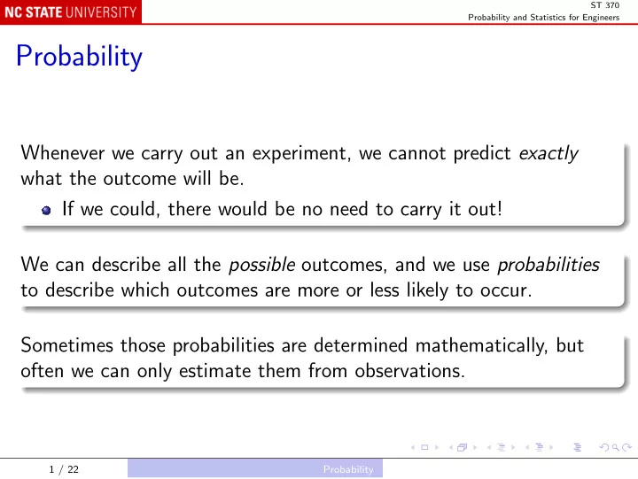
ST 370 Probability and Statistics for Engineers Probability Whenever we carry out an experiment, we cannot predict exactly what the outcome will be. If we could, there would be no need to carry it out! We can describe all the possible outcomes,
ST 370 Probability and Statistics for Engineers Probability Whenever we carry out an experiment, we cannot predict exactly what the outcome will be. If we could, there would be no need to carry it out! We can describe all the possible outcomes, and we use probabilities to describe which outcomes are more or less likely to occur. Sometimes those probabilities are determined mathematically, but often we can only estimate them from observations. 1 / 22 Probability
ST 370 Probability and Statistics for Engineers Example: Acceptance sampling A business receives a shipment of 200 electronic components, and one is chosen at random, and tested for compliance with its requirements. The two possible outcomes are “item is compliant” or “item is non-compliant”. Suppose the shipment contains 5 non-compliant items; the definition of “chosen at random” is that each item in the shipment has the same chance of being chosen, namely 1 in 200, or 0.005. So the probability that the chosen item is non-compliant is 5 in 200, or 0.025. 2 / 22 Probability
ST 370 Probability and Statistics for Engineers Example: Camera flash Suppose that the specifications for a cell phone camera flash require it to recharge in no longer than 0.6 seconds. A phone is chosen at random from a production line and tested for compliance; let p be the probability of being in compliance. We have no simple way to calculate p , but we could estimate it by testing a random sample of phones. Note These are objective probabilities: two engineers seeing the same data would agree on the probability; the probability that the next President will be a Republican is subjective , not objective. 3 / 22 Probability
ST 370 Probability and Statistics for Engineers Probabilities from counting Recall the shipment: 200 items, 5 non-compliant. Suppose two items are chosen at random: The first is equally likely to be any of the 200; The second is equally likely to be any of the remaining 199. What is the probability that exactly one of them is non-compliant? 4 / 22 Probability
ST 370 Probability and Statistics for Engineers Either: The first is non-compliant (probability = 5/200) and the second is compliant (probability = 195/199); or The first is compliant (probability = 195/200) and the second is non-compliant (probability = 5/199). So the probability is 200 × 195 5 199 + 195 5 5 × 195 200 × 199 = 2 × 200 × 199 = 0 . 048995 . This is an example of the hypergeometric distribution. 5 / 22 Probability
ST 370 Probability and Statistics for Engineers Conditional probability Recall the cell phone camera flash units. Suppose the flash intensity is also required to be at least 800 watt-seconds: A = recharge time ≤ 0 . 6 seconds; B = intensity ≥ 800 watt-seconds. Suppose that 90% of flash units have acceptable recharge time, and 99% of those have acceptable intensity. Then the percentage of acceptable units is 0 . 9 × 0 . 99 × 100% = 89 . 1%. 6 / 22 Probability
ST 370 Probability and Statistics for Engineers In terms of probabilities for a randomly chosen flash unit, the probability of an acceptable recharge time is 0 . 9; we write P ( A ) = 0 . 9 . Then given an acceptable recharge time, the probability of an acceptable intensity is 0 . 99; we write P ( B given A ) = 0 . 99 . This is the conditional probability of B given A , written P ( B | A ). 7 / 22 Probability
ST 370 Probability and Statistics for Engineers Complement of an event The event that A does not happen, the complement of A , is A ′ = not A = recharge time > 0 . 6 seconds; The probability is P ( A ′ ) = 1 − P ( A ) = 0 . 1 . Often, in solving problems, P ( A ′ ) is easier to calculate than P ( A ), and P ( A ) is found from P ( A ) = 1 − P ( A ′ ) . 8 / 22 Probability
ST 370 Probability and Statistics for Engineers Multiplication rule The flash unit is compliant if both recharge time and intensity are acceptable; the probability is P ( A and B ) = 0 . 9 × 0 . 99 = P ( A ) × P ( B | A ) . This is written P ( A ∩ B ): P ( A ∩ B ) = P ( A ) × P ( B | A ) . Consequently P ( B | A ) = P ( A ∩ B ) , P ( A ) which is sometimes taken as the definition of conditional probability. 9 / 22 Probability
ST 370 Probability and Statistics for Engineers Probabilistic independence Suppose that the percentage of flash units with acceptable intensity is the same 99%, regardless of whether the recharge time is acceptable: P ( B ) = 0 . 99 = P ( B | A ) . That is, the conditional probability P ( B | A ) is the same as the unconditional probability P ( B ). Then P ( A ∩ B ) = P ( A ) × P ( B | A ) = P ( A ) × P ( B ) . We say that A and B are independent (probabilistically, or stochastically). 10 / 22 Probability
ST 370 Probability and Statistics for Engineers It is easy to show that, when A and B are probabilistically independent, then also: A ′ and B are probabilistically independent; A and B ′ are probabilistically independent; A ′ and B ′ are probabilistically independent. 11 / 22 Probability
ST 370 Probability and Statistics for Engineers Note that non-compliance of difference aspects of the same unit are often not independent. For instance, a bad connection to a capacitor might lead to both slow recharge and low intensity. Often P (not B | not A ) = P ( B ′ | A ′ ) > P ( B ′ ) so that A ′ and B ′ are (probabilistically) dependent , not independent . We might sometimes assume, however, that compliance of a cell phone flash unit is (probabilistically) independent of compliance of the touch screen, for example if they are supplied from different sources. 12 / 22 Probability
ST 370 Probability and Statistics for Engineers Total probability Example: semiconductor manufacturing Chips are occasionally exposed to high levels of contamination ( H ), leading to an increased risk of failure ( F ): P ( F | H ) = 0 . 100 , P ( F | H ′ ) = 0 . 005 , P ( H ) = 0 . 2 . What is the probability of failure, P ( F )? 13 / 22 Probability
ST 370 Probability and Statistics for Engineers Failure can occur after high contamination, or not after high contamination, but not both, so P (Failure) = P (Failure and High contamination) + P (Failure and not High contamination) That is, P ( F ) = P ( F ∩ H ) + P ( F ∩ H ′ ) = P ( F | H ) P ( H ) + P ( F | H ′ ) P ( H ′ ) = 0 . 1 × 0 . 2 + 0 . 005 × (1 − 0 . 2) = 0 . 024 . 14 / 22 Probability
ST 370 Probability and Statistics for Engineers Bayes’ Rule Suppose that a chip is observed to fail. What is the probability that it was exposed to high level of contamination? That is, what is P ( H | F )? P ( H | F ) = P ( H ∩ F ) P ( F ) = P ( F | H ) P ( H ) P ( F ) = 0 . 1 × 0 . 2 0 . 024 = 0 . 833 . 15 / 22 Probability
ST 370 Probability and Statistics for Engineers Using the total probability expression for P ( F ), we could write P ( F | H ) P ( H ) P ( H | F ) = P ( F | H ) P ( H ) + P ( F | H ′ ) P ( H ′ ) which is the usual way to write Bayes’ rule. In general, more than two terms may appear in the denominator. For example, contamination could be Low ( C 1 ), Medium ( C 2 ), or High ( C 3 ), each with its own risk of subsequent failure: P ( F | C i ) P ( C i ) P ( C i | F ) = � 3 j =1 P ( F | C j ) P ( C j ) 16 / 22 Probability
ST 370 Probability and Statistics for Engineers Prior and posterior probabilities P ( C i ) is sometimes called the prior probability of C i , because it is known before we find out whether the chip fails. Similarly, P ( C i | F ) is called the posterior probability of C i , because it can be calculated after we find out that the chip has failed. Bayes’ rule shows how the information that the chip failed changes the probabilities of the levels of contamination: P ( F | C i ) P ( C i | F ) = P ( C i ) × � 3 j =1 P ( F | C j ) P ( C j ) 17 / 22 Probability
ST 370 Probability and Statistics for Engineers Odds ratio The odds on the event H that a chip is exposed to the high level of contamination are P ( H ) 1 − P ( H ) = 0 . 2 P ( H ) 0 . 8 = 1 P ( H ′ ) = 4 , or 1 : 4 . The posterior odds ratio, given that the chip failed, is P ( H ′ | F ) = P ( H ) P ( H | F ) P ( H ′ ) × P ( F | H ) P ( F | H ′ ) = 1 4 × 0 . 100 0 . 005 = 1 4 × 20 , or 5 : 1. 18 / 22 Probability
ST 370 Probability and Statistics for Engineers That is, posterior odds = prior odds × Bayes factor , where the “Bayes factor” is P ( F | H ) P ( F | H ′ ) . The Bayes factor is also known as the likelihood ratio , the ratio of the probabilities of what was observed (chip failure) given the two possible histories (contaminated versus uncontaminated). 19 / 22 Probability
ST 370 Probability and Statistics for Engineers A diagnostic testing example A certain population has a 1.48% prevalence of bowel cancer. The fecal occult blood screen test has 67% sensitivity and 91% specificity. A person is randomly chosen from the population, and tested. Write C for the event that the person suffers from the cancer, and T for the event that the test is positive for the presence of cancer. Then P ( C ) = 0 . 0148 (prevalence) P ( T | C ) = 0 . 67 (sensitivity) P ( T | C ′ ) = 1 − 0 . 91 = 0 . 09 (specificity) and hence P ( T ) = 0 . 67 × 0 . 0148 + 0 . 09 × (1 − 0 . 0148) = 0 . 0986 . 20 / 22 Probability
Recommend
More recommend
Explore More Topics
Stay informed with curated content and fresh updates.
