Probability Distributions and Introduction to Statistical Inference - PowerPoint PPT Presentation

Probability Distributions and Introduction to Statistical Inference BIO5312 FALL2017 STEPHANIE J. SPIELMAN, PHD

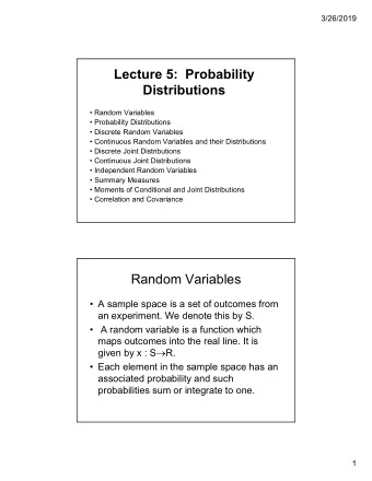
Random variable Random processes produce numerical outcomes: ◦ Number of tails in 50 coin flips ◦ The sum of everyone's heights Definition: a random variable is a function that maps outcomes of a random process to a numeric value ◦ X is a function (rule) that assign a number X(s) to each outcome s ∈ S (where s is an event in sample space S ) ◦ r.v.'s are technically neither random nor variables… ◦ But, you can think of them roughly numerical outcomes of random processes

Discrete vs continuous RV Discrete random variables can take on (map to) a finite number of values Continuous random variables can take on (map to) innumerable/infinite values

Expressing discrete random variables Probability mass function (PMF) ◦ Describes the values taken by a discrete r.v. X and its associated probabilities ◦ Function that assigns, to any possible value x of a discrete r.v. X , the probability P(X = x) PMF for rolling a fair die P(X = x) P( 0.15 Event probability 0.10 0.05 0.00 x 1 2 3 4 5 6 Event

�� PMF properties 0 ≤ 𝑄 𝑌 = 𝑦 ≤ 1 ∑ 𝑄 𝑌 = 𝑦 = 1 PMF is simply a fancier term for a discrete probability distribution

Expressing discrete random variables Cumulative distribution function (CDF) ◦ Function defined, for a specific value x of a discrete r.v. X , as F(x) = P(X ≤ x) CDF for rolling a fair die 1.00 0.75 Cumulative probability P(X ≤ 4 ) P( 0.50 0.25 P( P(X ≤ 1 ) 0.00 1 2 3 4 5 6 Event

CDF properties 0 ≤ 𝐺 𝑌 ≤ 1 CDF functions are non-decreasing

PMF vs CDF PMF: What is the probability of event X? CDF: What is the sum of probabilities for all events ≤ X?

� � Expectation and spread of random variables The expectation of a r.v. is the probability-weighted average of all possible values (i.e., mean) ◦ 𝔽 𝑌 = 𝜈 = ∑ 𝑦 / 𝑞(𝑦 / ) / The variance of a r.v. is defined ◦ 𝑊𝑏𝑠 𝑌 = 𝜏 7 = 𝔽[ 𝑌 − 𝜈 7 ] = ∑ [𝑦 / 7 𝑞(𝑦 / ) ] − 𝜈 7 / ◦ 𝑊𝑏𝑠 𝑌 = 𝔽[𝑌 7 ] − 𝔽[𝑌] 7

Example: The Binomial distribution The binomial distribution describes the probability of obtaining k successes in n Bernoulli trials, where the probability of success for each trial is constant at p A Bernoulli trial has a binary outcome (success/fail, true/false, yes/no), and P(success) = p is the same for all realizations of the trial

The BInS conditions To be binomially distributed, must satisfy the following: B inary outcomes I ndependent trials (outcomes do not influence each other) n is fixed before the trials begin S ame probability of success, p, for all trials

Is it binomial? A bag contains 10 balls, 7 red and 3 green. Situation 1: You draw 5 balls from the bag, noting the ball color each time and then returning it to the bag. Yes! Situation 2: You draw 5 balls from the bag, retaining each drawn ball for safe-keeping so you can play catch at any moment. No L Situation 3: You keep drawing balls, with replacement, until you have drawn 4 red balls. No L

The binomial distribution The PMF (probability distribution) for a binomially- distributed random variable: < < = 𝑞 = (1 − 𝑞) (<>=) = = 𝑞 = 𝑟 (<>=) 𝑄 𝑌 = 𝑙 = <! The binomial coefficient: < = = =! <>= ! ◦ read as "n choose k"

Wikipedia weighs in

The binomial distribution The expectation for a binomial r.v. ◦ 𝔽 𝑌 = 𝜈 = np The variance for a binomial r.v. ◦ 𝑊𝑏𝑠 𝑌 = 𝜏 7 = npq = np(1 − p) We write binomially distributed r.v.'s as 𝑌~𝐶(𝑜, 𝑞)

Example: Playing with a binomial rv Each child born to a particular set of parents has a 25% probability of having blood type O. Assume the parents had five children. Here, n = 5 and p = 0.25, meaning we define Type O as "success", and not Type O as "failure". à X~B(5, 0.25) Tasks: ◦ Compute expectation and variance ◦ Visualize PMF ◦ Visualize CDF ◦ Make some calculations…

Expectation and variance Each child born to a particular set of parents has a 25% probability of having blood type O. Assume the parents had five children. B(5, 0.25) 𝔽 𝑌 = 𝜈 = np = 5*0.25 = 1.25 𝑊𝑏𝑠 𝑌 = 𝜏 7 = npq = np(1 − p) = 5*0.25*0.75 = 0.9375

Visualize the PMF 0.3955078125 0.4 Probability Type O 0.3 0.263671875 0.2373046875 0.2 0.1 0.087890625 0.0146484375 0.0009765625 0.0 0 1 2 3 4 5 Number of kids

?distributions Distributions in the stats package Description: Density, cumulative distribution function, quantile function and random variate generation for many standard probability distributions are available in the ‘stats’ package. Details: The functions for the density/mass function, cumulative distribution function, quantile function and random variate generation are named in the form ‘dxxx’, ‘pxxx’, ‘qxxx’ and ‘rxxx’ respectively. For the beta distribution see ‘dbeta’. For the binomial (including Bernoulli) distribution see ‘dbinom’. For the Cauchy distribution see ‘dcauchy’. For the chi-squared distribution see ‘dchisq’.

Distribution functions, generally Function Purpose Binomial version dxxx() dxxx() dbinom(x, size, prob) Probability distribution pbinom(q, size, prob) pxxx pxxx() () CDF rxxx rxxx() () Generate random rbinom(n, size, prob) numbers from given distribution qxxx qxxx() () qbinom(p, size, prob) Quantile: Inverse of pxxx()

Binomial distribution functions Binomial function Example Output dbinom(x, size, prob) dbinom(2, 5, 0.25) Prob of obtaining 2 successes in 5 trials, where p=0.25 à 0.263 pbinom(q, size, prob) pbinom(2, 5, 0.25) Prob of obtaining ≤2 successes in 5 trials, where p=0.25 à 0.896 rbinom(n, size, prob) rbinom(100, 5, 0.25) Generate 100 k values from this binomial dist. à 100 from {0,1,2,3,4} qbinom(p, size, prob) qbinom(0.896, 5, 0.25) Smallest value x where F(x) >= p* à 2 *not prob success, just a prob

0.4 0.3955078125 Probability Type O 0.3 0.263671875 0.2373046875 0.2 Making the PMF 0.1 0.087890625 0.0146484375 0.0009765625 0.0 0 1 2 3 4 5 Number of kids > ## Use dbinom() to get the PMF values > p = 0.25 > n = 5 > k0 <- dbinom(0, 5, 0.25) ## Prob of 0 successes, aka no children are Type O > k1 <- dbinom(1, 5, 0.25) ## Prob of 1 success, aka only 1 child is Type O > ## Advanced: > library(purrr) > map_dbl(0:5, dbinom, 5, 0.25) [1] 0.2373046875 0.3955078125 0.2636718750 0.0878906250 0.0146484375 [6] 0.0009765625

Making the PMF ## data frame (tibble) of probabilities for PMF > data.pmf <- tibble(k = 0:5, prob = c(0.236623, 0.396, 0.264, 0.0879, 0.0145, 0.000977)) > data.pmf # A tibble: 6 x 2 k prob <int> <dbl> 1 0 0.236623 2 1 0.396000 3 2 0.264000 4 3 0.087900 5 4 0.014500 6 5 0.000977 ## Equivalent > data.pmf <- tibble(k = 0:5, prob = map_dbl(0:5, dbinom, 5, 0.25))

Making the PMF uses a different *stat* > ggplot(data.pmf, aes(x = k, y=prob))+ geom_bar( stat="identity" ) + xlab("Number of kids") + ylab("Probability Type O") 0.4 0.3 Probability Type O 0.2 0.1 0.0 0 2 4 Number of kids

Tweaking the x-axis > ggplot(data.pmf, aes(x = k, y=prob))+ geom_bar( stat="identity" ) + ylab("Probability Type O") + scale_x_continuous(name = "Number of kids", breaks = 0:5) 0.4 0.3 Probability Type O 0.2 0.1 0.0 0 1 2 3 4 5 Number of kids

Adding some text > ggplot(data.pmf, aes(x = k, y=prob))+ geom_bar( stat="identity" ) + ylab("Probability Type O") + scale_x_continuous(name = "Number of kids", breaks = 0:5) + geom_text(aes(x = k, y= prob + 0.01, label = prob)) 0.396 0.4 Probability Type O 0.3 0.264 0.236623 0.2 0.1 0.0879 0.0145 0.000977 0.0 0 1 2 3 4 5 Number of kids

Visualize the CDF > binom.sample <- tibble(x = rbinom(1000, 5, 0.25)) > ggplot(binom.sample, aes(x=x)) + stat_ecdf() + xlab("# Type O kids") + ylab("Cumulative probability") 1.00 Cumulative probability 0.75 0.50 0.25 0.00 0 1 2 3 4 5 # Type O kids

Solving for probabilities Each child born to a particular set of parents has a 25% probability of having blood type O. Assume the parents had five children. B(5, 0.25) What is the probability that exactly 2 children were Type O? 0.4 0.3955078125 > dbinom(2, 5, 0.25) [1] 0.2636719 Probability Type O 0.3 0.263671875 0.2373046875 0.2 0.1 0.087890625 0.0146484375 0.0009765625 0.0 0 1 2 3 4 5 Number of kids

Solving for probabilities Each child born to a particular set of parents has a 25% probability of having blood type O. Assume the parents had five children. B(5, 0.25) What is the probability that exactly 2 children were Type O? 0.4 0.3955078125 𝑄 𝑌 = 𝑙 = 𝑜 𝑙 𝑞 = (1 − 𝑞) (<>=) = 𝑜 𝑙 𝑞 = 𝑟 (<>=) Probability Type O 0.3 0.263671875 0.2373046875 0.2 I 7 0.25 7 0.75 (I>7) 𝑄 𝑌 = 2 = 0.1 0.087890625 = 10 * 0.0625 * 0.422 = 0.26375 0.0146484375 0.0009765625 0.0 0 1 2 3 4 5 Number of kids