Probability Definitions Probability Space : ordered triple ( , F , P - PDF document

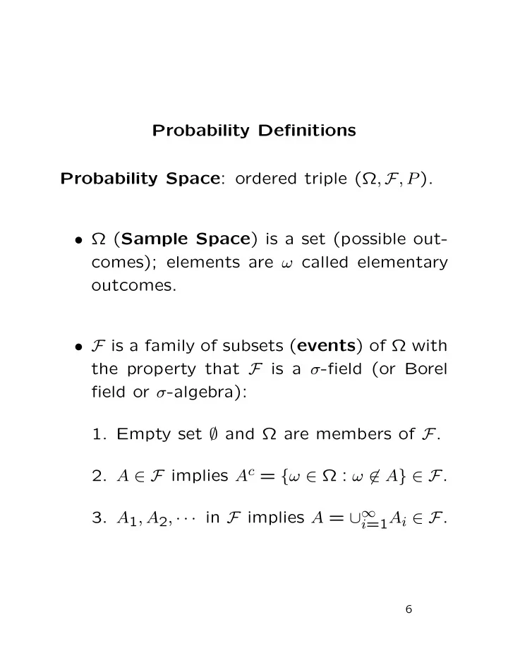
Probability Definitions Probability Space : ordered triple (Ω , F , P ). • Ω ( Sample Space ) is a set (possible out- comes); elements are ω called elementary outcomes. • F is a family of subsets ( events ) of Ω with the property that F is a σ -field (or Borel field or σ -algebra): 1. Empty set ∅ and Ω are members of F . 2. A ∈ F implies A c = { ω ∈ Ω : ω �∈ A } ∈ F . 3. A 1 , A 2 , · · · in F implies A = ∪ ∞ i =1 A i ∈ F . 6

• P a function, domain F , range a subset of [0 , 1] satisfying: 1. P ( ∅ ) = 0 and P (Ω) = 1. 2. Countable additivity : A 1 , A 2 , · · · pair- wise disjoint ( j � = k A j ∩ A k = ∅ ) ∞ P ( ∪ ∞ � i =1 A i ) = P ( A i ) i =1 Axioms guarantee can compute probabilities by usual rules, including approximation. Consequences of axioms: A i ∈ F ; i = 1 , 2 , · · · implies ∩ i A i ∈ F A 1 ⊂ A 2 ⊂ · · · implies P ( ∪ A i ) = lim n →∞ P ( A n ) A 1 ⊃ A 2 ⊃ · · · implies P ( ∩ A i ) = lim n →∞ P ( A n ) 7

Vector valued random variable : function X : Ω �→ R p such that, writing X = ( X 1 , . . . , X p ), P ( X 1 ≤ x 1 , . . . , X p ≤ x p ) defined for any const’s ( x 1 , . . . , x p ). Formally X 1 ≤ x 1 , . . . , X p ≤ x p is a subset of Ω or event : { ω ∈ Ω : X 1 ( ω ) ≤ x 1 , . . . , X p ( ω ) ≤ x p } . X is ftn on Ω so X 1 also ftn on Ω. Almost always dependence of random variable on ω hidden: see X not X ( ω ). Jargon and notation: we write P ( X ∈ A ) for P ( { ω ∈ Ω : X ( ω ) ∈ A } ) and define the distri- bution of X to be the map A �→ P ( X ∈ A ) (Probability on R p not on original Ω.) 8

(CDF) Cumulative Distribution Function of X : function F X on R p defined by F X ( x 1 , . . . , x p ) = P ( X 1 ≤ x 1 , . . . , X p ≤ x p ) . Properties of F X (usually just F ) for p = 1: 1. 0 ≤ F ( x ) ≤ 1. 2. x > y ⇒ F ( x ) ≥ F ( y ) (monotone non- decreasing). 3. lim x →−∞ F ( x ) = 0 and lim x →∞ F ( x ) = 1. 4. lim x ց y F ( x ) = F ( y ) (right continuous). 5. lim x ր y F ( x ) ≡ F ( y − ) exists. 6. F ( x ) − F ( x − ) = P ( X = x ). 7. F X ( t ) = F Y ( t ) for all t implies that X and Y have the same distribution, that is, P ( X ∈ A ) = P ( Y ∈ A ) for any (Borel) set A . 9

Defn : Distribution of rv X is discrete (also call X discrete) if ∃ countable set x 1 , x 2 , · · · such that � P ( X ∈ { x 1 , x 2 · · · } ) = 1 = P ( X = x i ) . i In this case the discrete density or probability mass function of X is f X ( x ) = P ( X = x ) . Defn : Distribution of rv X is absolutely con- tinuous if there is a function f such that � P ( X ∈ A ) = A f ( x ) dx (1) for any (Borel) set A . This is a p dimensional integral in general. Equivalently � x F ( x ) = −∞ f ( y ) dy . Defn : Any f satisfying (1) is a density of X . For most x F is differentiable at x and F ′ ( x ) = f ( x ) . 10

Example : X is Uniform[0,1].  0 x ≤ 0   F ( x ) = 0 < x < 1 x 1 x ≥ 1 .    1 0 < x < 1   f ( x ) = undefined x ∈ { 0 , 1 } 0 otherwise .   Density CDF 0.8 0.8 density 0.0 0.0 -1.0 0.0 0.5 1.0 1.5 2.0 -1.0 0.0 0.5 1.0 1.5 2.0 Example : X is exponential. 1 − e − x � x > 0 F ( x ) = x ≤ 0 . 0 e − x  x > 0   f ( x ) = undefined x = 0 0 x < 0 .   Density CDF 0.8 0.8 density 0.0 0.0 0 2 4 6 0 2 4 6 11