On the measurement of frequency and of its sample variance with - PowerPoint PPT Presentation

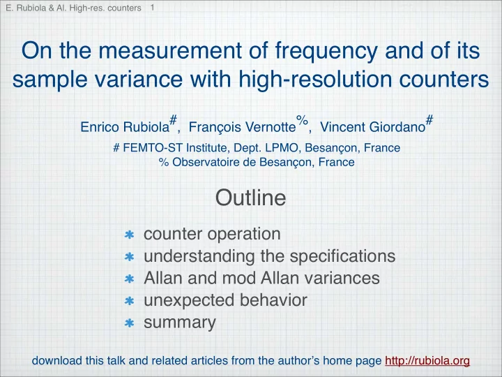
1 E. Rubiola & Al. High-res. counters On the measurement of frequency and of its sample variance with high-resolution counters Enrico Rubiola#, François Vernotte%, Vincent Giordano# # FEMTO-ST Institute, Dept. LPMO, Besançon, France % Observatoire de Besançon, France Outline counter operation understanding the specifications Allan and mod Allan variances unexpected behavior summary download this talk and related articles from the author ’ s home page http://rubiola.org

2 E. Rubiola & Al. High-res. counters frequency stability measurement direct measurement beat method (increased resolution) ν (t) ν b (t) ν (t) counter counter ν c ν c frequency reference frequency reference y ( t ) = ν ( t ) − ν 00 fractional frequency fluctuation ν 00 σ 2 � y ( t ) 2 � y = E classical variance � 1 � 2 � � σ 2 y ( τ ) = E Allan variance y k +1 − y k 2

E. Rubiola & Al. High-res. counters 3 classical reciprocal counter (1) measurement. time M pulses τ = N/ ν Μ = τν c ν ÷N binary counter trigger ν c N ν c readout = ν reference M period measurement (count the clock pulses) is preferred to frequency measurement (count the input pulses) because: it provides higher resolution in a given measurement time tau (the clock frequency can be close to the maximum switching speed) interpolation (M is rational instead of integer) can be used to reduce the quantization (interpolators only work at a fixed frequency, thus at the clock freq.)

classical reciprocal counter (2) phase time x x 0 x 1 x 2 x 3 x N (i.e., time jitter) v(t) time t 4 t 0 t 1 t 2 t 3 t 4 t 5 t 6 t N period T 00 weight 1/τ w Π 0 measurement time τ = NT � + ∞ E { ν } = ν ( t ) w Π ( t ) dt Π estimator measure: scalar product −∞ � 1 /τ 0 < t < τ w Π ( t ) = weight 0 elsewhere � + ∞ w Π ( t ) dt = 1 normalization −∞ y = 2 σ 2 variance σ 2 x classical variance τ 2

5 E. Rubiola & Al. High-res. counters enhanced-resolution counter n − 1 phase time x E { ν } = 1 x 0 x 1 x 2 x 3 x N � (i.e., time jitter) ν i ν i = N/τ i n v(t) time i =0 t t 0 t 1 t 2 t 3 t 4 t 5 t 6 t N − D t N t N+D meas. no. Λ estimator 1/ τ w 0 0 i = 0 � + ∞ w 1 i = 1 E { ν } = ν ( t ) w Λ ( t ) dt w 2 weight i = 2 −∞ w i weight  w n − 1 t/τ 0 < t < τ i = n − 1   w Λ ( t ) = 2 − t/τ τ < t < 2 τ delay τ 0 = DT measurement time τ = NT = nDT  0 elsewhere  1 n − 1 n − 1 normalization τ n τ n τ � + ∞ 2 2 weight 1 1 w Λ w Λ ( t ) dt = 1 n τ n τ n τ n τ −∞ white noise: the autocorrelation limit τ 0 -> 0 of the weight function function is a narrow pulse, about 1/ τ the inverse of the bandwidth w Λ (t) 2 σ 2 y = 1 t classical the variance is 0 σ 2 τ 2 τ x τ 2 variance divided by n n

6 E. Rubiola & Al. High-res. counters understanding technical information y = 2 σ 2 classical classical reciprocal σ 2 x τ 2 variance counter enhanced-resolution 2 σ 2 y = 1 classical σ 2 x τ 2 counter variance n low frequency: τ 0 = T = n = ν 00 τ ⇒ full speed 2 σ 2 1 classical σ 2 x y = τ 3 ν 00 variance high frequency: τ 0 = DT with D> 1 = n = ν 00 τ ⇒ housekeeping takes time 2 σ 2 y = 1 classical x σ 2 τ 3 ν I variance the slope of the classical variance tells the whole story 1 /τ 2 = Π estimator (classical reciprocal) ⇒ 1 /τ 3 = Λ estimator (enhanced-resolution) ⇒ look for formulae and plots in the instruction manual

7 E. Rubiola & Al. High-res. counters examples Stanford SRS-620 � �� 2 � 2 � �� � � � � (25 ps) 2 + short term gate trigger + 2 × � � � × RMS stability time jitter frequency = resolution N gate time (in Hz) RMS resolution σ ν = ν 00 σ y frequency ν 00 gate time τ Agilent 53132A � � ( t res ) 2 + 2 × ( trigger error ) 2 � � � 4 × t jitter � � RMS frequency = + × ( gate time ) × √ or period resolution no. of samples gate time t res = 225 ps t jitter = 3 ps � (gate time) × (frequency) for f < 200 kHz number of samples = (gate time) × 2 × 10 5 for f ≥ 200 kHz RMS resolution σ ν = ν 00 σ y or σ T = T 00 σ y frequency ν 00 period T 00 gate time τ � ν 00 < 200 kHz ν 00 τ no. of samples n = τ × 2 × 10 5 ν 00 ≥ 200 kHz

8 E. Rubiola & Al. High-res. counters Allan variance � 1 � 2 � � σ 2 y ( τ ) = E definition y k +1 − y k 2 � ( k +2) τ � ( k +1) τ � � 2 � 1 � 1 y ( t ) dt − 1 σ 2 y ( τ ) = E y ( t ) dt 2 τ τ ( k +1) τ kτ ��� + ∞ � 2 � wavelet-like σ 2 y ( τ ) = E y ( t ) w A ( t ) dt variance −∞ w 1 A  1 0 < t < τ √ − 2 τ 2 τ time   0 1 w A = τ < t < 2 τ √ t 2 τ − 1  0 elsewhere  2 τ 0 τ 2 τ � + ∞ A ( t ) dt = 1 the Allan variance differs from a wavelet variance in w 2 energy E { w A } = the normalization on power, instead of on energy τ −∞

9 E. Rubiola & Al. High-res. counters modified Allan variance � 1 � ( i +2 n ) τ 0 � ( i + n ) τ 0 n − 1 � �� 2 � 1 � 1 y ( t ) dt − 1 � definition mod σ 2 y ( τ ) = E y ( t ) dt 2 n τ τ ( i + n ) τ 0 iτ 0 i =0 with τ = n τ 0 . ��� + ∞ � 2 � mod σ 2 y ( τ ) = E y ( t ) w M ( t ) dt −∞ wavelet-like  variance 1 0 < t < τ 2 τ 2 t √ −  1  w  1  2 τ 2 (2 t − 3) τ < t < 2 τ M  √ 2 τ w M = time 1 � 2 τ 2 ( t − 3 2 τ < t < 3 τ 0 √ −  3 τ t  τ 2 τ  − 1  0 elsewhere  0 2 τ � + ∞ M ( t ) dt = 1 w 2 E { w M } = energy 2 τ −∞ E { w M } = 1 compare the energy 2 E { w A } this explains why the mod Allan variance is always lower than the Allan variance

10 E. Rubiola & Al. High-res. counters spectra and variances noise σ 2 mod σ 2 S ϕ ( f ) S y ( f ) y ( τ ) y ( τ ) S ϕ ↔ S y type 3 f H h 2 (2 π ) 2 τ − 2 3 f H τ 0 h 2 white h 2 = b 0 τ − 3 h 2 f 2 b 0 PM ν 2 (2 π ) 2 0 2 πτ f H ≫ 1 flicker h 1 = b − 1 h 1 0 . 084 h 1 τ − 2 (2 π ) 2 τ − 2 b − 1 f − 1 [1 . 038+3 ln(2 π f H τ )] h 1 f PM ν 2 n ≫ 1 0 1 1 white h 0 = b − 2 2 h 0 τ − 1 4 h 0 τ − 1 b − 2 f − 2 h 0 FM ν 2 0 27 flicker h − 1 = b − 3 h − 1 f − 1 b − 3 f − 3 2 ln(2) h − 1 20 ln(2) h − 1 FM ν 2 0 random (2 π ) 2 0 . 824 (2 π ) 2 h − 2 = b − 4 b − 4 f − 4 h − 2 f − 2 walk h − 2 τ h − 2 τ ν 2 6 6 FM 0 1 1 2 D 2 y τ 2 2 D 2 y τ 2 frequency drift ˙ y = D y ν 00 is replaced with ν 0 for consistency with the general literature. f H is the high cuto ff frequency, needed for the noise power to be finite.

11 E. Rubiola & Al. High-res. counters classical counter —> Allan variance given a series of contiguous non-overlapped measures measure series t ν 0 ν 1 ν 2 ν 3 ...... ...... 1/ τ time w Π (t) t 1/ τ w Π (t − ) τ t +1/( 2 τ ) w (t) A − 1/( 2 τ ) t 0 τ 2 τ the Allan variance is easily evaluated � 1 � 2 � � σ 2 y ( τ ) = E y k +1 − y k 2

12 E. Rubiola & Al. High-res. counters enhanced-resolut. counter —> Allan variance by feeding a series of Λ -estimates of frequency in the formula of the Allan variance � 1 � 2 � � σ 2 y ( τ ) = E y k +1 − y k 2 as they were Π -estimates t ..... ..... ν 0 ν 1 ν 2 ν 3 1/ τ time w Λ (t) t 1/ τ w Λ (t − ) τ t +1/( 2 τ ) w (t) M − 1/( 2 τ ) t 0 τ 2 τ 3 τ one gets exactly the modified Allan variance! � 1 � ( i +2 n ) τ 0 � ( i + n ) τ 0 n − 1 � �� 2 � � 1 1 y ( t ) dt − 1 � mod σ 2 y ( τ ) = E y ( t ) dt 2 n τ τ ( i + n ) τ 0 iτ 0 i =0 with τ = n τ 0 .

13 E. Rubiola & Al. High-res. counters joining contiguous values to increase τ graphical proof mod Allan τ = τ B (1) w t m=2 t τ =2 τ B (2) w t m=4 t τ =4 τ B w (3) t m=8 t converges to Allan τ =8 τ B w (4) t m = 1 mod Allan m = 2 this is not what we expected m = 4 ... m ≥ 8 the variance converges to the (non modified) Allan variance

14 E. Rubiola & Al. High-res. counters Summary in frequency measurements, the Λ (triangular) estimator provides higher resolution the Λ estimator can not be used in time-interval measurements mistakes are around the corner if the counter inside is not well understood manufacturers, please provide full technical information for your instruments Thanks to J. Dick (JPL), C. Greenhall (JPL), D. Howe (NIST) and M. Oxborrow (NPL) for stimulating discussion, to the open-software community for providing almost all what we needed, up-to-date, reliable and free To know more: 1 - rubiola.org, slides and articles 2 - www.arxiv.org, document arXiv:physics/0503022v1 3 - Rev. of Sci. Instrum. vol. 76 no. 5, art.no. 054703, May 2005.

15 E. Rubiola & Al. High-res. counters actual formulae look like this σ y = 1 � 2( δ t ) 2 trigger + 2( δ t ) 2 (Π) interpolator τ 1 � 2( δ t ) 2 trigger + 2( δ t ) 2 (Λ) σ y = τ √ n interpolator � ν 0 τ ν 00 ≤ ν I n = ν 00 > ν I ν I τ