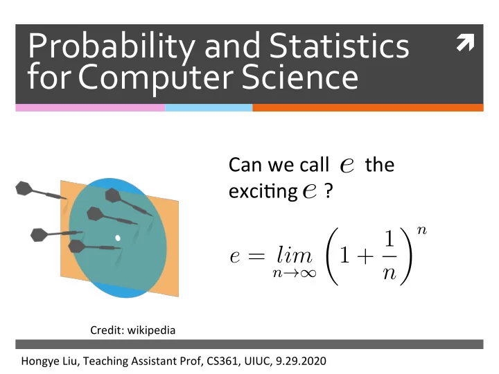

Probability and Statistics ì for Computer Science Can we call the e exci-ng ? e � n � 1 + 1 e = lim n n →∞ Credit: wikipedia Hongye Liu, Teaching Assistant Prof, CS361, UIUC, 9.29.2020
Last time
Objectives ✺ Poisson distribu-on ✺ Con-nuous Random Variable ✺ Uniform Con-nuous distribu-on ✺ Exponen-al distribu-on
Motivation for a model called Poisson Distribution ✺ What’s the probability of the number of incoming customers (k) in an hour? ✺ It’s widely applicable in physics and engineering both for modeling of -me and space. Simeon D. Poisson Credit: wikipedia (1781-1840)
Poisson Distribution ✺ A discrete random variable X is called Poisson with intensity λ (λ>0) if P ( X = k ) = e − λ λ k k ! for integer k ≥ 0 λ is the average rate of Simeon D. Poisson x the event ′ s occurrence (1781-1840)
Poisson Distribution ✺ Poisson distribu-on is a valid pdf for ∞ ∞ λ i λ k e − λ � i ! = e λ ⇒ � = 1 k ! i =0 k =0 P ( X = k ) = e − λ λ k k ! for integer k ≥ 0 λ is the average rate of Simeon D. Poisson x the event ′ s occurrence (1781-1840)
Poisson Distribution ✺ Poisson distribu-on is a valid pdf for ∞ ∞ λ i λ k e − λ � i ! = e λ ⇒ � = 1 x k ! i =0 k =0 P ( X = k ) = e − λ λ k k ! for integer k ≥ 0 λ is the average rate of Simeon D. Poisson x the event ′ s occurrence (1781-1840)
Expectations of Poisson Distribution ✺ The expected value and the variance are wonderfully the same! That is λ P ( X = k ) = e − λ λ k k ! for integer k ≥ 0 E [ X ] = λ x var [ X ] = λ Simeon D. Poisson (1781-1840)
Examples of Poisson Distribution ✺ How many calls does a call center get in an hour? ✺ How many muta-ons occur per 100k nucleo-des in an DNA strand? ✺ How many independent incidents occur in an interval? P ( X = k ) = e − λ λ k k ! for integer k ≥ 0
Poisson Distribution: call center ✺ If a call center receives 10 calls per hour on average, what is the probability that it receives 15 calls in a given hour? ✺ What is λ here? ✺ What is P(k=15)? Credit: wikipedia
Q. Poisson Distribution: call center If a call center receives 4 calls per hour on average. What is intensity λ here for an hour? A. 1 B. 4 C. 8 Credit: wikipedia
Q. Poisson Distribution: call center If a call center receives 4 calls per hour on average. What is probability the center receives 0 calls in an hour? A. e -4 B. 0.5 C. 0.05 Credit: wikipedia
Q. Poisson Distribution: call center ✺ Given a call center receives 10 calls per hour on average, what is the intensity λ of the distribu-on for calls in Two hours? Credit: wikipedia
Example of a continuous random variable ✺ The spinner θ θ ∈ (0 , 2 π ] 0 ✺ The sample space for all outcomes is not countable
Probability density function (pdf) ✺ For a con-nuous random variable X, the probability that X = x is essen-ally zero for all (or most) x , so we can’t define P ( X = x ) ✺ Instead, we define the probability density func;on (pdf) over an infinitesimally small interval dx, p ( x ) dx = P ( X ∈ [ x, x + dx ]) � b ✺ For a < b p ( x ) dx = P ( X ∈ [ a, b ]) a
Properties of the probability density function ✺ resembles the probability func-on p ( x ) of discrete random variables in that ✺ for all x p ( x ) ≥ 0 ✺ The probability of X taking all possible values is 1. � ∞ p ( x ) dx = 1 −∞
Properties of the probability density function ✺ differs from the probability p ( x ) distribu-on func-on for a discrete random variable in that ✺ is not the probability that X = x p ( x ) ✺ can exceed 1 p ( x )
Probability density function: spinner ✺ Suppose the spinner has equal chance stopping at any posi-on. What’s the pdf of the angle θ of the spin posi-on? c � if θ ∈ (0 , 2 π ] c p ( θ ) = 0 otherwise 0 2π θ ✺ For this func-on to be a pdf, Then � ∞ p ( θ ) d θ = 1 −∞
Probability density function: spinner ✺ What the probability that the spin angle θ is within [ ]? 12 , π π 7
Q: Probability density function: spinner ✺ What is the constant c given the spin angle θ has the following pdf? p ( θ ) A. 1 B. 1/π C. 2/π c D. 4/π E. 1/2π π 0 2π θ
Expectation of continuous variables ✺ Expected value of a con-nuous random variable X weight � ∞ E [ X ] = xp ( x ) dx x −∞ ✺ Expected value of func-on of con-nuous random variable Y = f ( X ) � ∞ E [ Y ] = E [ f ( X )] = f ( x ) p ( x ) dx −∞
Probability density function: spinner ✺ Given the probability density of the spin angle θ � 1 if θ ∈ (0 , 2 π ] p ( θ ) = 2 π 0 otherwise ✺ The expected value of spin angle is � ∞ E [ θ ] = θ p ( θ ) d θ −∞
Properties of expectation of continuous random variables ✺ The linearity of expected value is true for con-nuous random variables. � � ✺ And the other proper-es that we derived for variance and covariance also hold for con-nuous random variable
Q. ✺ Suppose a con-nuous variable has pdf � 2(1 − x ) x ∈ [0 , 1] p ( x ) = 0 otherwise What is E[X]? A. 1/2 B. 1/3 C. 1/4 D. 1 E. 2/3 � ∞ E [ X ] = xp ( x ) dx −∞
Continuous uniform distribution ✺ A con-nuous random variable X is uniform if p ( x ) 1 b − a 1 0 a b X
Continuous uniform distribution ✺ A con-nuous random variable X is p ( x ) uniform if 1 b − a 1 1 � for x ∈ [ a, b ] p ( x ) = b − a 0 a 0 b X otherwise & var [ X ] = ( b − a ) 2 E [ X ] = a + b 2 12
Continuous uniform distribution ✺ A con-nuous random variable X is p ( x ) uniform if 1 b − a 1 1 � for x ∈ [ a, b ] p ( x ) = b − a 0 a 0 b X otherwise & var [ X ] = ( b − a ) 2 E [ X ] = a + b 2 12 ✺ Examples: 1) A dart’s posi-on thrown on the target
Continuous uniform distribution ✺ A con-nuous random variable X is p ( x ) uniform if 1 b − a 1 1 � for x ∈ [ a, b ] p ( x ) = b − a 0 a 0 b X otherwise & var [ X ] = ( b − a ) 2 E [ X ] = a + b 2 12 ✺ Examples: 1) A dart’s posi-on thrown on the target 2) Olen associated with random sampling
Cumulative distribution of continuous uniform distribution ✺ Cumula-ve distribu-on func-on (CDF) � x P ( X ≤ x ) = p ( x ) dx −∞ of a uniform random variable X is: CDF p ( x ) 1 1 b − a 1 0 a 0 a b X b X
Exponential distribution ✺ Common p ( x ) = λ e − λ x for x ≥ 0 Model for wai-ng -me ✺ Associated with the Poisson distribu-on with the same λ Credit: wikipedia
Exponential distribution ✺ A con-nuous random variable X is exponen-al if it represent the “-me” un-l next incident in a Poisson distribu-on with intensity λ . Proof See Morris et al Pg 324. p ( x ) = λ e − λ x for x ≥ 0 ✺ It’s similar to Geometric distribu;on – the discrete version of wai-ng in queue ✺ Both are memory-less. See Degroot et al Pg 322
Exponential distribution ✺ A con-nuous random variable X is exponen-al if it represent the “-me” un-l next incident in a Poisson distribu-on with intensity λ . Proof See Morris et al Pg 324. p ( x ) = λ e − λ x for x ≥ 0 ✺ It’s similar to Geometric distribu;on – the discrete version of wai-ng in queue
Expectations of Exponential distribution ✺ A con-nuous random variable X is exponen-al if it represent the “-me” un-l next incident in a Poisson distribu-on with intensity λ . p ( x ) = λ e − λ x for x ≥ 0 E [ X ] = 1 & var [ X ] = 1 x λ 2 λ
Example of exponential distribution ✺ How long will it take un-l the next call to be received by a call center? Suppose it’s a random variable T . If the number of incoming call is a Poisson distribu-on with intensity λ = 20 in an hour . What is the expected -me for T?
Q: ✺ A store has a number of customers coming on Sat. that can be modeled as a Poisson distribu-on. In order to measure the average rate of customers in the day, the staff recorded the -me between the arrival of customers, can he reach the same goal? A. Yes B. No
Normal (Gaussian) distribution ✺ The most famous con-nuous random variable distribu-on. The probability density is this: 2 π exp ( − ( x − µ ) 2 1 p ( x ) = ) √ 2 σ 2 σ E [ X ] = µ & var [ X ] = σ 2 Carl F. Gauss (1777-1855) Credit: wikipedia
Normal (Gaussian) distribution ✺ The most famous con-nuous random variable distribu-on. ? 2 π exp ( − ( x − µ ) 2 1 p ( x ) = ) √ 2 σ 2 σ E [ X ] = µ & var [ X ] = σ 2 Carl F. Gauss (1777-1855) Credit: wikipedia
Normal (Gaussian) distribution ✺ The most famous con-nuous random variable distribu-on. ? 2 π exp ( − ( x − µ ) 2 1 p ( x ) = ) √ 2 σ 2 σ � + ∞ p ( x ) dx = 1 −∞ E [ X ] = µ & var [ X ] = σ 2 Carl F. Gauss (1777-1855) Credit: wikipedia
Normal (Gaussian) distribution ✺ A lot of data in nature are approximately normally distributed, ie. Adult height , etc. 2 π exp ( − ( x − µ ) 2 1 p ( x ) = ) √ 2 σ 2 σ E [ X ] = µ & var [ X ] = σ 2 Carl F. Gauss (1777-1855) Credit: wikipedia
Spread of normal (Gaussian) distributed data 99.7% 95% 68% Credit: wikipedia
Recommend
More recommend