Probability, Statistics and Inference Probability : an abstract - PDF document

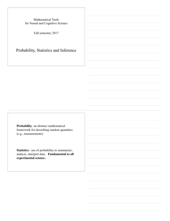
Mathematical Tools for Neural and Cognitive Science Fall semester, 2017 Probability, Statistics and Inference Probability : an abstract mathematical framework for describing random quantities (e.g., measurements) Statistics : use of probability to summarize, analyze, interpret data. Fundamental to all experimental science.

Probabilistic Middleville In Middleville, every family has two children, brought by the stork. The stork delivers boys and girls randomly, with equal l e d o m c probability. i s t l i b i a o b r p You pick a family at random and discover that one of the data children is a girl. What is the probability that the other child is a girl? statistical inference Statistical Middleville In Middleville, every family has two children, brought by the stork. The stork delivers boys and girls randomly, with equal probability. In a survey of 100 Middleville families, 32 have two girls, 24 have two boys, and the remainder have one of each. You pick a family at random and discover that one of the children is a girl. What is the probability that the other child is a girl?

- Efron & Tibshirani, Introduction to the Bootstrap Some historical context • 1600’s: Early notions of data summary/averaging • 1700’s: Bayesian prob/statistics (Bayes, Laplace) • 1920’s: Frequentist statistics for science (e.g., Fisher) • 1940’s: Statistical signal analysis and communication, estimation/decision theory (Shannon, Wiener, etc) • 1970’s: Computational optimization and simulation (e.g,. Tukey) • 1990’s: Machine learning (large-scale computing + statistical inference + lots of data) • Since 1950’s: statistical neural/cognitive models

Scientific process Observe / measure data Generate predictions, Summarize/fit , design experiment compare with predictions Create/modify hypothesis/model Estimating model parameters • How do I compute the estimate? 
 (mathematics vs. numerical optimization) • How “good” are my estimates? • How well does my model explain the data? 
 Future data (prediction/generalization)? • How do I compare two (or more) models?

Outline of what’s coming Themes: • Uni-variate vs. multi-variate • Discrete vs. continuous • Math vs. simulation • Bayesian vs. frequentist inference Topics: • Descriptive statistics • Basic probability theory: univariate, multivariate • Model parameter estimation • Hypothesis testing / model comparison Example: Localization Issues: Mean and variability (accuracy and precision)

Descriptive statistics: Central tendency • We often summarize data with the average. Why? • Average minimizes the squared error (think regression!) N N 1 x ) 2 = 1 X X arg min ( x n − ˆ x n N N ˆ x n =1 n =1 • More generally, for L p norms: # 1 /p N " 1 X x | p | x n − ˆ • minimum L 1 norm: median N i =1 • minimum L 0 norm: mode • Issues: Data from a common source, outliers, asymmetry, bimodality Descriptive statistics: Dispersion N 1 ( ) • Sample variance s 2 = ∑ 2 x i − x N − 1 i = 1 • Why N -1? • Sample standard deviation N • Mean absolute deviation 1 ∑ x i − x N i = 1

Example: Localization x ≠ 0 I find that . Is that convincing? Is the apparent bias real? To answer this, we need tools from probability… Probability: notation let X , Y, Z be random variables they can take on values (like ‘heads’ or ‘tails’; or integers 1-6; or real-valued numbers) let x, y, z stand generically for values they can take, and also, in shorthand, for events like X = x we write the probability that X takes on value x as P ( X = x ), or P X (x), or sometimes just P ( x ) P ( x ) is a function over x, which we call the probability “distribution” function (pdf) (or, for continuous variables only, “density”)

Discrete pdf Continuous pdf A distribution Another distribution (the sum of 2 dice rolls) (IQ or a randomly chosen person) P ( x ) p ( x ) Normalization p ( x ) P ( x ) 0 < P ( x ) < 1 0 < p ( x ) ∑ P ( x i ) = 1 ∞ ∫ p ( x ) dx = 1 i −∞

Probability basics • discrete probability distributions • continuous probability densities • cumulative distributions • translation and scaling of distributions • monotonic nonlinear transformations • drawing samples from a distribution. Uniform. Inverse cumulative mapping • example densities/distributions [on board] Example distributions a not-quite-fair coin roll of a fair die sum of two rolled fair dice 0.7 0.2 0.2 0.6 0.15 0.15 0.5 0.4 0.1 0.1 0.3 0.2 0.05 0.05 0.1 0 0 0 1 2 3 4 5 6 2 3 4 5 6 7 8 9 10 11 12 0 1 clicks of a Geiger counter, horizontal velocity of gas ... and, time between clicks in a fixed time interval molecules exiting a fan 0.25 0.1 0.2 0.08 0.15 0.06 0.1 0.04 0.05 0.02 0 0 1 2 3 4 5 6 7 8 9 10 11 0 200 400 600 800 1000 - 0 1 2 3 4 5 6 7 8 9 10

Expected value - discrete N ∑ E ( X ) = x i p ( x i ) [the mean, ] µ i = 1 10 4 2.5 0.7 0.6 2 0.5 1.5 # of students 0.4 P(x) 0.3 1 0.2 0.5 0.1 0 0 0 1 2 3 4 0 1 2 3 4 # of credit cards # of credit cards Expected value - continuous Z [the mean, ] E ( x ) = x p ( x ) dx µ Z x 2 p ( x ) dx E ( x 2 ) = [the “second moment”] Z ( x − µ ) 2 p ( x ) dx [the variance, ] σ 2 ( x − µ ) 2 � � = E Z x 2 p ( x ) dx − µ 2 = Z note: an inner product, E ( f ( x )) = f ( x ) p ( x ) dx and thus linear, i.e., E ( af ( X ) + bg ( X )) = aE ( f ( X )) + bE ( g ( X ))

Joint and conditional probability - discrete Joint and conditional probability - discrete P(Ace) P(Heart) P(Ace & Heart) “Independence” P(Ace | Heart) P(not Jack of Diamonds) P(Ace | not Jack of Diamonds)

Multi-variate probability • Joint distributions • Marginals (integrating) • Conditionals (slicing) • Bayes’ Rule (inverting) • Statistical independence (separability) [on board]

Marginal distribution p ( x, y ) Z p ( x ) = p ( x, y ) dy Conditional probability A B A & B Neither A nor B p ( A | B ) = probability of A given that B is asserted to be true = p ( A & B ) p ( B )

Conditional distribution p ( x, y ) p ( x | y = 68) Conditional distribution P(x|Y=68) �Z p ( x | y = 68) = p ( x, y = 68) p ( x, y = 68) dx - - . = p ( x, y = 68) p ( y = 68) More generally: p ( x | y ) = p ( x, y ) /p ( y ) slice joint distribution normalize (by marginal)

Bayes’ Rule A B A & B p ( A | B ) = probability of A given that B is asserted to be true = p ( A & B ) p ( B ) p ( A & B ) = p ( B ) p ( A | B ) = p ( A ) p ( B | A ) ⇒ p ( A | B ) = p ( B | A ) p ( A ) p ( B ) Bayes’ Rule p ( x | y ) = p ( y | x ) p ( x ) /p ( y ) (a direct consequence of the definition of conditional probability)

Conditional vs. marginal P ( x | Y =120) - P ( x ) - In general, these differ. When are they they same? In particular, when are all conditionals equal to the marginal? Statistical independence Random variables X and Y are statistically independent if (and only if): p ( x , y ) = p ( x ) p ( y ) ∀ x , y [note: for discrete distributions, this is an outer product!] Independence implies that all conditionals are equal to the corresponding marginal: p ( x | y ) = p ( x , y ) / p ( y ) = p ( x ) ∀ x , y

Sums of independent RVs For any two random variables (independent or not): E ( X + Y ) = E ( X ) + E ( Y ) Suppose X and Y are independent, then E ( XY ) = E ( X ) E ( Y ) ( ) ⎛ ( ) − µ X + µ Y ( ) ⎞ 2 + σ Y 2 σ X + Y 2 = E X + Y ⎠ = σ X 2 ⎝ p X + Y ( z ) and is a convolution Implications: (1) Sums of Gaussians are Gaussian, (2) Properties of the sample average Mean and variance • Mean and variance summarize centroid/width • translation and rescaling of random variables • nonlinear transformations - “warping” • Mean/variance of weighted sum of random variables • The sample average • ... converges to true mean (except for bizarre distributions) • ... with variance • ... most common common choice for an estimate ...

Point Estimates • Estimator: Any function of the data, intended to compute an estimate of the true value of a parameter • The most common estimator is the sample average, used to estimate the true mean of the distribution. • Statistically-motivated examples: - Maximum likelihood (ML): - Max a posteriori (MAP): - Min Mean Squared Error 
 (MMSE): Example: Estimate the bias of a coin

Bayes’ Rule and Estimation Posterior Likelihood Prior p (parameter value |data) = p (data | parameter value) p (parameter value) p (data) Nuisance normalizing term

Likelihood: 1 head Likelihood: 1 tail Posteriors, p(H,T|x), assuming prior p(x)=1 More tails T=0 1 2 3 More heads H=0 1 2 3

example infer whether a coin is fair by flipping it repeatedly here, x is the probability of heads (50% is fair) y 1. ..n are the outcomes of flips Consider three different priors: suspect fair suspect biased no idea prior fair prior biased prior uncertain X likelihood (heads) = posterior

previous posteriors X likelihood (heads) = new posterior previous posteriors X likelihood (tails) = new posterior

Posteriors after observing 75 heads, 25 tails à prior differences are ultimately overwhelmed by data Confidence PDFs 2H / 1T 10H / 5T 20H / 10T CDFs .975 .025 .19 .93 .49 .80