Probability 2: Random variables and Expectations E [ X + Y ] = E [ X - PowerPoint PPT Presentation
15-251: Great Theoretical Ideas in Computer Science Fall 2016 Lecture 18 October 27, 2016 Probability 2: Random variables and Expectations E [ X + Y ] = E [ X ] + E [ Y ] Review Some useful sample spaces 1) A fair coin sample space =
15-251: Great Theoretical Ideas in Computer Science Fall 2016 Lecture 18 October 27, 2016 Probability 2: Random variables and Expectations E [ X + Y ] = E [ X ] + E [ Y ]
Review Some useful sample spaces …
1) A fair coin sample space Ω = {H, T} Pr[H] = ½ , Pr[T] = ½. 2) A “bias - p” coin sample space Ω = {H, T} Pr[H] = p, Pr[T] = 1-p.
3) Two independent bias-p coin tosses sample space Ω = {HH, HT, TH, TT} Pr x x 2 T T , 1 p , 1 T H p p , 1 H T p p 2 H H , p
3) n bias-p coins sample space Ω = {H,T} n If outcome x in Ω has k heads and n-k tails Pr[x] = p k (1-p) n-k Event E k = {x ∈ Ω | x has k heads} 𝑜 𝑙 𝑞 𝑙 1 − 𝑞 𝑜−𝑙 Pr 𝐹 𝑙 = Pr 𝑦 = 𝑦∈𝐹 𝑙 𝑜 “Binomial Distribution B( n,p) 𝑙 𝑞 𝑙 1 − 𝑞 𝑜−𝑙 Pr 𝑙 = on {0,1,2,…,n}”
An Infinite sample space…
The “Geometric” Distribution A bias-p coin is tossed until the first time that a head turns up. sample space Ω = {H, TH, TTH, TTTH, …} (shorthand Ω = {1, 2, 3, 4, …}) (1-p) k-1 p Pr Geom [k] = (sanity check) k≥1 Pr[k] = k≥1 (1-p) k-1 p = p * (1 + (1-p) + (1-p) 2 + …) = p * 1/(1-(1-p)) = 1
Independence of Events def: We say events A, B are independent if Pr [A∩B] = Pr [A] Pr [B] Except in the pointless case of Pr [A] or Pr [B] is 0, equivalent to Pr [A | B] = Pr [A], or to Pr [B | A] = Pr [B].
Two fair coins are flipped A = {first coin is heads} B = {second coin is heads} Are A and B independent? Pr[A] = Pr[B] = H,H H,T Pr[A B] = T,H T,T
Two fair coins are flipped A = {first coin is heads} C = {two coins have different outcomes} Are A and C independent? Pr[A] = Pr[C] = H,H H,T Pr[A | C] = T,H T,T
Two fair coins are flipped A = {first coin is heads} A = {first coin is tails} Are A and A independent? H,H H,T T,H T,T
The Secret “Principle of Independence” Suppose you have an experiment with two parts (eg. two non-interacting blocks of code). A … Suppose A is an event that only depends on the first part, B B only on the second part. Suppose you prove that the two parts cannot affect each other. (E.g., equivalent to run them in opposite order.) Then A and B are independent. And you may deduce that Pr [A | B] = Pr [A].
Independence of Multiple Events def: A 1 , …, A 5 are independent if Pr [A 1 ∩A 2 ∩A 3 ∩A 4 ∩A 5 ] = Pr [A 1 ] Pr [A 2 ] Pr [A 3 ] Pr [A 4 ] Pr [A 5 ] & Pr [A 1 ∩A 2 ∩A 3 ∩A 4 ] = Pr [A 1 ] Pr [A 2 ] Pr [A 3 ] Pr [A 4 ] & Pr [A 1 ∩A 3 ∩A 5 ] = Pr [A 1 ] Pr [A 3 ] Pr [A 5 ] & in fact, the definition requires
Independence of Multiple Events def: A 1 , …, A 5 are independent if Similar ‘ Principle of Independence ’ holds (5 blocks of code which don’t affect each other) Consequence: anything like
A little exercise Can you give an example of a sample space and 3 events 𝐵 1 , 𝐵 2 , 𝐵 3 in it such that each pair of events 𝐵 𝑗 , 𝐵 𝑘 are independent, but 𝐵 1 , 𝐵 2 , 𝐵 3 together aren’t independent?
Feature Presentation: Random Variables
Random Variable Let Ω be sample space in a probability distribution A Random Variable is a function from Ω to reals Examples: F = value of first die in a two-dice roll F (3,4) = 3, F (1,6) = 1 X = sum of values of the two dice X (3,4) = 7, X (1,6) = 7
Two Coins Tossed Z : {TT, TH, HT, HH} → {0, 1, 2} counts the number of heads Induces distribution on {0,1,2} Ω HH 2 ¼ ¼ TT ¼ 0 ¼ TH ¼ 1 HT ½ ¼
Two Coins Tossed Z : {TT, TH, HT, HH} → {0, 1, 2} counts # of heads Pr[ Z = a] = Z Ω HH 2 Pr[{t Ω | Z (t) = a}] ¼ ¼ TT 0 ¼ ¼ TH Pr[ Z = 1] ¼ 1 ½ HT = Pr[{t Ω | Z (t) = 1}] ¼ Distribution = Pr[{TH, HT}] = ½ of Z
Two Views of Random Variables Input to the function is Think of a R.V. as random A function from sample space to the reals R Or think of the induced distribution on R Randomness is “pushed” to the values of the function Given a distribution on some sample space Ω , a random variable transforms it into a distribution on reals
Two dice X = sum of both dice I throw a white die and a black die . Sample space = 1/5 { (1,1), (1,2), (1,3), (1,4), (1,5), (1,6), 3/20 (2,1), (2,2), (2,3), (2,4), (2,5), (2,6), (3,1), (3,2), (3,3), (3,4), (3,5), (3,6), 1/10 (4,1), (4,2), (4,3), (4,4), (4,5), (4,6), 1/20 (5,1), (5,2), (5,3), (5,4), (5,5), (5,6), 0 2 3 4 5 6 7 8 9 10 11 12 (6,1), (6,2), (6,3), (6,4), (6,5), (6,6) } Distribution of X function with X (1,1) = 2, X (1,2) = 3, …, X (6,6)=12
Random variables: two viewpoints It is a function on the sample space It is a variable with a probability distribution on its values You should be comfortable with both views
Random Variables: introducing them Retroactively: “Let D be the random variable given by subtracting the first roll from the second.” D ( (1,1) ) = 0, …, D ( (5, 3) ) = −2, etc.
Random Variables: introducing them In terms of other random variables: ⇒ “Let Y = X 2 + D .” Y ( (5,3) ) = 62 “Suppose you win $30 on a roll of double -6, and you lose $1 otherwise. Let W be the random variable representing your winnings.” W = 30 ∙ I + (-1) (1- I) = 31 ∙ I − 1 Where I ((6,6))=1 and I ((x,y))=0 otherwise
Random Variables: introducing them By describing its distribution: “Let X be a Bernoulli(1/3) random variable .” • Means Pr[ X =1]=1/3, Pr[ X =0]=2/3 “Let Y be a Binomial(100,1/3) random variable.” “Let T be a random variable which is uniformly distributed (= each value equal probability) on the set {0,2,4,6,8 }.”
Random Variables to Events E.g.: S = sum of two dice “Let A be the event that S ≥ 10.” A = { (4,6), (5,5), (5,6), (6,4), (6,5), (6,6) } Pr [ S ≥ 10] = 6/36 = 1/6 Shorthand notation for the event { ℓ : S (ℓ) ≥ 10 }.
Events to Random Variables Definition: Let A be an event. The indicator of A is the random variable X which is 1 when A occurs and 0 when A doesn’t occur. X : Ω → ℝ
Notational Conventions Use letters like A, B, C for events Use letters like X, Y, f, g for R.V.’s R.V. = random variable
Independence of Random Variables Definition: Random variables X and Y are independent if the events “ X = u ” and “ Y = v ” are independent for all u,v ∈ℝ . (And similarly for more than 2 random variables.) Random variables X 1 , X 2 , …, X n are independent if for all reals a 1 , a 2 , …, a n
Examples: Independence of r.v’s Two random variables X and Y are said to be independent if for all reals a, b, Pr[ X = a Y = b] = Pr[ X =a] Pr[ Y =b] A coin is tossed twice. X i = 1 if the i th toss is heads and 0 otherwise. Are X 1 and X 2 independent R.Vs ? Yes. Let Y = X 1 +X 2 . Are X 1 and Y independent? No.
Expectation aka Expected Value aka Mean
Expectation Intuitively, expectation of X is what its average value would be if you ran the experiment millions and millions of times. Definition: Let X be a random variable in experiment with sample space Ω . Its expectation is:
Expectation — examples Let R be the roll of a standard die. = 3.5 Question: What is Pr [ R = 3.5]? Answer: 0. Don’t always expect the expected!
Expectation — examples “Suppose you win $30 on a roll of double -6, and you lose $1 otherwise. Let W be the random variable representing your winnings.” = −5/36 ≈ −13.9¢
Expectation — examples Let R 1 = Throw of die 1, R 2 = Throw of die 2 S = R 1 + R 2 . = lots of arithmetic = 7 (eventually)
One of the top tricks in probability...
Linearity of Expectation Given an experiment, let X and Y be any random variables. Then E [ X + Y ] = E [ X ] + E [ Y ] X and Y do not have to be independent!!
Linearity of Expectation E [ X + Y ] = E [ X ] + E [ Y ] Proof: Let Z = X + Y (another random variable). Then
Linearity of Expectation E [ X + Y ] = E [ X ] + E [ Y ] Also: E [a X +b] = a E [ X ]+b for any a,b ∈ℝ . By Induction E [ X 1 + ∙∙∙ + X n ] = E [ X 1 ] + ∙∙∙ + E [ X n ]
Remember… E[X 1 + X 2 + … + X n ] = E[X 1 ] + E[X 2 ] + …. + E[ X n ], always The expectation of the sum = The sum of the expectations
Linearity of Expectation example Let R 1 = Throw of die 1, R 2 = Throw of die 2 S = R 1 + R 2 . = 3.5 + 3.5 = 7
Expectation of an Indicator Fact: Let A be an event, let X be its indicator r.v. Then E [ X ] = Pr [A]. Proof:
Linearity of Expectation + Indicators = best friends forever
Linearity of Expectation + Indicators There are 251 students in a class. The TAs randomly permute their midterms before handing them back. Let X be the number of students getting their own midterm back. What is E [ X ]?
Let’s try 3 students first # getting Student 1 Student 2 Student 3 Prob own midterm 1 2 3 1/6 3 Midterm they got 1 3 2 1/6 1 2 1 3 1/6 1 2 3 1 1/6 0 3 1 2 1/6 0 3 2 1 1/6 1 ∴ E [ X ] = (1/6)(3+1+1+0+0+1) = 1
Now let’s do 251 students Um…
Recommend
More recommend
Explore More Topics
Stay informed with curated content and fresh updates.
