Power, Sample Size, and the FDR Peter Dalgaard Department of - PowerPoint PPT Presentation

Power, Sample Size, and the FDR Peter Dalgaard Department of Biostatistics University of Copenhagen Center for Bioinformatics, Univ.Copenhagen, June 2005

Sample Size “How many observations do we need?” Depends on • Design • Standard error of measurements • Effect size • How sure you want to be of finding it

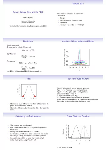
Sample Size “How many observations do we need?” Depends on • Design • Standard error of measurements • Effect size • How sure you want to be of finding it

Sample Size “How many observations do we need?” Depends on • Design • Standard error of measurements • Effect size • How sure you want to be of finding it

Sample Size “How many observations do we need?” Depends on • Design • Standard error of measurements • Effect size • How sure you want to be of finding it

Sample Size “How many observations do we need?” Depends on • Design • Standard error of measurements • Effect size • How sure you want to be of finding it

Reminders (Continuous data) One-sample (or paired, differences): � SEM = s × 1 / n Significance if | ¯ x − µ 0 | > t . 975 ( DF ) SEM Two-sample: � SEDM = s × 1 / n 1 + 1 / n 2 | ¯ x 1 − ¯ x 2 | SEDM > t . 975 ( DF ) t . 975 ( DF ) ≈ 2. Notice that SE(D)M decreases with n .

Reminders (Continuous data) One-sample (or paired, differences): � SEM = s × 1 / n Significance if | ¯ x − µ 0 | > t . 975 ( DF ) SEM Two-sample: � SEDM = s × 1 / n 1 + 1 / n 2 | ¯ x 1 − ¯ x 2 | SEDM > t . 975 ( DF ) t . 975 ( DF ) ≈ 2. Notice that SE(D)M decreases with n .

Reminders (Continuous data) One-sample (or paired, differences): � SEM = s × 1 / n Significance if | ¯ x − µ 0 | > t . 975 ( DF ) SEM Two-sample: � SEDM = s × 1 / n 1 + 1 / n 2 | ¯ x 1 − ¯ x 2 | SEDM > t . 975 ( DF ) t . 975 ( DF ) ≈ 2. Notice that SE(D)M decreases with n .

Reminders (Continuous data) One-sample (or paired, differences): � SEM = s × 1 / n Significance if | ¯ x − µ 0 | > t . 975 ( DF ) SEM Two-sample: � SEDM = s × 1 / n 1 + 1 / n 2 | ¯ x 1 − ¯ x 2 | SEDM > t . 975 ( DF ) t . 975 ( DF ) ≈ 2. Notice that SE(D)M decreases with n .

Reminders (Continuous data) One-sample (or paired, differences): � SEM = s × 1 / n Significance if | ¯ x − µ 0 | > t . 975 ( DF ) SEM Two-sample: � SEDM = s × 1 / n 1 + 1 / n 2 | ¯ x 1 − ¯ x 2 | SEDM > t . 975 ( DF ) t . 975 ( DF ) ≈ 2. Notice that SE(D)M decreases with n .

Variation of Observations and Means dnorm(x, sd = sqrt(1/20)) 1.5 1.0 0.5 0.0 −3 −2 −1 0 1 2 3 x

t Test 0.4 0.3 dt(t, 38) 0.2 0.1 0.0 −3 −2 −1 0 1 2 3 t • If there is no (true) difference then there is little chance of getting an observation in the tails • If there is a difference, then the center of the distribution is shifted.

t Test 0.4 0.3 dt(t, 38) 0.2 0.1 0.0 −3 −2 −1 0 1 2 3 t • If there is no (true) difference then there is little chance of getting an observation in the tails • If there is a difference, then the center of the distribution is shifted.

Type I and Type II Errors A test of a hypothesis can go wrong in two ways: Type I error: Rejecting a true null hypothesis Type II error: Accepting a false null hypothesis Error probabilities: α resp. β α : Significance level (0.05, e.g.) 1 − β : Power – probability of detecting difference Notice that the power depends on the effect size as well as on the number of observations and significance level.

Type I and Type II Errors A test of a hypothesis can go wrong in two ways: Type I error: Rejecting a true null hypothesis Type II error: Accepting a false null hypothesis Error probabilities: α resp. β α : Significance level (0.05, e.g.) 1 − β : Power – probability of detecting difference Notice that the power depends on the effect size as well as on the number of observations and significance level.

Type I and Type II Errors A test of a hypothesis can go wrong in two ways: Type I error: Rejecting a true null hypothesis Type II error: Accepting a false null hypothesis Error probabilities: α resp. β α : Significance level (0.05, e.g.) 1 − β : Power – probability of detecting difference Notice that the power depends on the effect size as well as on the number of observations and significance level.

Type I and Type II Errors A test of a hypothesis can go wrong in two ways: Type I error: Rejecting a true null hypothesis Type II error: Accepting a false null hypothesis Error probabilities: α resp. β α : Significance level (0.05, e.g.) 1 − β : Power – probability of detecting difference Notice that the power depends on the effect size as well as on the number of observations and significance level.

Calculating n – Preliminaries • (First consider one-sample case) • Wish to find difference of δ = µ − µ 0 (“clinically relevant difference”), • Naive guess: n should satisfy δ = 2 × SEM? • But the observed difference is not precisely δ . It is smaller with 50% probability, and then it wouldn’t be significant. • We need to make SEM so small that there is a high probability of getting a significant result

Calculating n – Preliminaries • (First consider one-sample case) • Wish to find difference of δ = µ − µ 0 (“clinically relevant difference”), • Naive guess: n should satisfy δ = 2 × SEM? • But the observed difference is not precisely δ . It is smaller with 50% probability, and then it wouldn’t be significant. • We need to make SEM so small that there is a high probability of getting a significant result

Calculating n – Preliminaries • (First consider one-sample case) • Wish to find difference of δ = µ − µ 0 (“clinically relevant difference”), • Naive guess: n should satisfy δ = 2 × SEM? • But the observed difference is not precisely δ . It is smaller with 50% probability, and then it wouldn’t be significant. • We need to make SEM so small that there is a high probability of getting a significant result

Calculating n – Preliminaries • (First consider one-sample case) • Wish to find difference of δ = µ − µ 0 (“clinically relevant difference”), • Naive guess: n should satisfy δ = 2 × SEM? • But the observed difference is not precisely δ . It is smaller with 50% probability, and then it wouldn’t be significant. • We need to make SEM so small that there is a high probability of getting a significant result

Calculating n – Preliminaries • (First consider one-sample case) • Wish to find difference of δ = µ − µ 0 (“clinically relevant difference”), • Naive guess: n should satisfy δ = 2 × SEM? • But the observed difference is not precisely δ . It is smaller with 50% probability, and then it wouldn’t be significant. • We need to make SEM so small that there is a high probability of getting a significant result

Power, Sketch of Principle 0.4 0.3 dnorm(x) 0.2 0.1 0.0 −2 0 2 4 6 x (x axis in units of SEM)

Size of SEM relative to δ (Notice: These formulas assume known SD. Watch out if n is very small. More accurate formulas in R’s power.t.test ) z p quantiles in normal distribution, z 0 . 975 = 1 . 96, etc. Two-tailed test, α = 0 . 05, power 1 − β = 0 . 90 δ = ( 1 . 96 + k ) × SEM k is distance between middle and right peak in slide 8. Find k so that there is a probability of 0.90 of observing a difference of at least 1 . 96 × SEM. k = − z 0 . 10 = z 0 . 90 z 0 . 90 = 1 . 28, so δ = 3 . 24 × SEM

Size of SEM relative to δ (Notice: These formulas assume known SD. Watch out if n is very small. More accurate formulas in R’s power.t.test ) z p quantiles in normal distribution, z 0 . 975 = 1 . 96, etc. Two-tailed test, α = 0 . 05, power 1 − β = 0 . 90 δ = ( 1 . 96 + k ) × SEM k is distance between middle and right peak in slide 8. Find k so that there is a probability of 0.90 of observing a difference of at least 1 . 96 × SEM. k = − z 0 . 10 = z 0 . 90 z 0 . 90 = 1 . 28, so δ = 3 . 24 × SEM

Size of SEM relative to δ (Notice: These formulas assume known SD. Watch out if n is very small. More accurate formulas in R’s power.t.test ) z p quantiles in normal distribution, z 0 . 975 = 1 . 96, etc. Two-tailed test, α = 0 . 05, power 1 − β = 0 . 90 δ = ( 1 . 96 + k ) × SEM k is distance between middle and right peak in slide 8. Find k so that there is a probability of 0.90 of observing a difference of at least 1 . 96 × SEM. k = − z 0 . 10 = z 0 . 90 z 0 . 90 = 1 . 28, so δ = 3 . 24 × SEM

Calculating n Just insert SEM = σ/ √ n in δ = 3 . 24 × SEM and solve for n : n = ( 3 . 24 × σ/δ ) 2 (for two-sided test at level α = 0 . 05, with power 1 − β = 0 . 90) General formula for arbitrary α and β : n = (( z 1 − α/ 2 + z 1 − β ) × ( σ/δ )) 2 = ( σ/δ ) 2 × f ( α, β ) next slide

Calculating n Just insert SEM = σ/ √ n in δ = 3 . 24 × SEM and solve for n : n = ( 3 . 24 × σ/δ ) 2 (for two-sided test at level α = 0 . 05, with power 1 − β = 0 . 90) General formula for arbitrary α and β : n = (( z 1 − α/ 2 + z 1 − β ) × ( σ/δ )) 2 = ( σ/δ ) 2 × f ( α, β ) next slide