Posterior odds interpretation of a sigmoid Artificial Intelligence: - PDF document

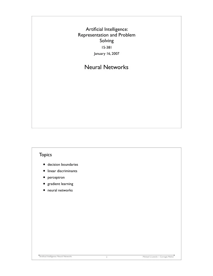
Artificial Intelligence: Representation and Problem Solving 15-381 January 16, 2007 Neural Networks Topics • decision boundaries • linear discriminants • perceptron • gradient learning • neural networks Artificial Intelligence: Neural Networks Michael S. Lewicki � Carnegie Mellon 2

The Iris dataset with decision tree boundaries 2.5 2 petal width (cm) 1.5 1 0.5 0 1 2 3 4 5 6 7 petal length (cm) Artificial Intelligence: Neural Networks Michael S. Lewicki � Carnegie Mellon 3 The optimal decision boundary for C 2 vs C 3 • optimal decision boundary is p ( petal length | C 3 ) determined from the statistical p ( petal length | C 2 ) 0.9 distribution of the classes 0.8 0.7 • optimal only if model is correct � 0.6 0.5 • assigns precise degree of uncertainty 0.4 0.3 to classification 0.2 0.1 0 2.5 2 petal width (cm) 1.5 1 0.5 0 1 2 3 4 5 6 7 petal length (cm) Artificial Intelligence: Neural Networks Michael S. Lewicki � Carnegie Mellon 4

Optimal decision boundary Optimal decision boundary p ( C 2 | petal length ) p ( C 3 | petal length ) 1 0.8 p ( petal length | C 2 ) p ( petal length | C 3 ) 0.6 0.4 0.2 0 1 2 3 4 5 6 7 Artificial Intelligence: Neural Networks Michael S. Lewicki � Carnegie Mellon 5 Can we do better? • only way is to use more information p ( petal length | C 3 ) • DTs use both petal width and petal p ( petal length | C 2 ) 0.9 0.8 length 0.7 0.6 0.5 0.4 0.3 0.2 0.1 0 2.5 2 petal width (cm) 1.5 1 0.5 0 1 2 3 4 5 6 7 petal length (cm) Artificial Intelligence: Neural Networks Michael S. Lewicki � Carnegie Mellon 6

Arbitrary decision boundaries would be more powerful 2.5 Decision boundaries could be non-linear 2 petal width (cm) 1.5 1 0.5 0 1 2 3 4 5 6 7 petal length (cm) Artificial Intelligence: Neural Networks Michael S. Lewicki � Carnegie Mellon 7 Defining a decision boundary • consider just two classes 2.5 • want points on one side of line in class 1, otherwise class 2. • 2D linear discriminant function: 2 x 2 m T x + b y = 1.5 m 1 x 1 + m 2 x 2 + b = � m i x i + b = i 1 • This defines a 2D plane which 3 4 5 6 7 x 1 leads to the decision: The decision boundary : y = m T x + b = 0 � class 1 if y ≥ 0, x ∈ class 2 if y < 0. Or in terms of scalars: m 1 x 1 + m 2 x 2 − b = − m 1 x 1 + b ⇒ x 2 = m 2 Artificial Intelligence: Neural Networks Michael S. Lewicki � Carnegie Mellon 8

Linear separability • Two classes are linearly separable if they can be separated by a linear combination of attributes - 1D: threshold - 2D: line not linearly separable - 3D: plane - M-D: hyperplane 2.5 2 petal width (cm) 1.5 1 0.5 linearly separable 0 1 2 3 4 5 6 7 petal length (cm) Artificial Intelligence: Neural Networks Michael S. Lewicki � Carnegie Mellon 9 Diagraming the classifier as a “neural” network • The feedforward neural network is specified by weights w i and bias b : y “output unit” w T x + b y = b “bias” M � w i x i + b w 1 w 2 w M “weights” = i =1 x 1 x 2 x M “input units” • • � • • It can written equivalently as M y � y = w T x = w i x i i =0 w 0 w 1 w 2 w M • where w 0 = b is the bias and a “dummy” input x 0 that is always 1 . x 1 x 2 x M • • � • x 0 =1 Artificial Intelligence: Neural Networks Michael S. Lewicki � Carnegie Mellon 10

Determining, ie learning, the optimal linear discriminant • First we must define an objective function , ie the goal of learning • Simple idea: adjust weights so that output y( x n ) matches class c n • Objective : minimize sum-squared error over all patterns x n : N E = 1 � ( w T x n − c n ) 2 2 n =1 • Note the notation x n defines a pattern vector : x n = { x 1 , . . . , x M } n • We can define the desired class as: � 0 x n ∈ class 1 c n = 1 x n ∈ class 2 Artificial Intelligence: Neural Networks Michael S. Lewicki � Carnegie Mellon 11 We’ve seen this before: curve fitting t = sin(2 π x ) + noise t n t 1 y ( x n , w ) 0 � 1 x x n 0 1 example from Bishop (2006), Pattern Recognition and Machine Learning Artificial Intelligence: Neural Networks Michael S. Lewicki � Carnegie Mellon 12

Neural networks compared to polynomial curve fitting M y ( x, w ) = w 0 + w 1 x + w 2 x 2 + · · · + w M x M = � w j x j N j =0 E ( w ) = 1 � [ y ( x n , w ) − t n ] 2 2 n =1 1 1 0 0 � 1 � 1 For the linear network, M=1 and 0 1 0 1 there are multiple input dimensions 1 1 0 0 � 1 � 1 0 1 0 1 example from Bishop (2006), Pattern Recognition and Machine Learning Artificial Intelligence: Neural Networks Michael S. Lewicki � Carnegie Mellon 13 General form of a linear network • A linear neural network is simply a y linear transformation of the input. M � W y j = w i,j x i i =0 x • Or, in matrix-vector form: y = Wx y i y K y 1 “outputs” • • � • • • � • • Multiple outputs corresponds to multivariate regression “weights” w ij x 1 x i x M x 0 =1 • • � • • • � • “inputs” “bias” Artificial Intelligence: Neural Networks Michael S. Lewicki � Carnegie Mellon 14

Training the network: Optimization by gradient descent • We can adjust the weights incrementally to minimize the objective function. • This is called gradient descent • Or gradient ascent if we’re maximizing. • The gradient descent rule for weight w i is: i − �∂ E w t +1 = w t i w i w 2 w 4 • Or in vector form: w 3 w t +1 = w t − �∂ E w 2 w • For gradient ascent , the sign w 1 of the gradient step changes. w 1 Artificial Intelligence: Neural Networks Michael S. Lewicki � Carnegie Mellon 15 Computing the gradient • Idea: minimize error by gradient descent • Take the derivative of the objective function wrt the weights: N 1 � ( w T x n − c n ) 2 = E 2 n =1 N ∂ E 2 � = ( w 0 x 0 ,n + · · · + w i x i,n + · · · + w M x M,n − c n ) x i,n w i 2 n =1 N � ( w T x n − c n ) x i,n = n =1 • And in vector form: N ∂ E � ( w T x n − c n ) x n w = n =1 Artificial Intelligence: Neural Networks Michael S. Lewicki � Carnegie Mellon 16

Simulation: learning the decision boundary • Each iteration updates the gradient: 2.5 i − �∂ E w t +1 = w t i 2 w i x 2 N ∂ E 1.5 � ( w T x n − c n ) x i,n = w i n =1 1 3 4 5 6 7 • Epsilon is a small value: x 1 11000 � = 0.1/N 10000 Learning Curve 9000 8000 • Epsilon too large: 7000 Error - learning diverges 6000 5000 • Epsilon too small: 4000 3000 - convergence slow 2000 1000 0 5 10 15 iteration Artificial Intelligence: Neural Networks Michael S. Lewicki � Carnegie Mellon 17 Simulation: learning the decision boundary • Each iteration updates the gradient: 2.5 i − �∂ E w t +1 = w t i 2 w i x 2 N ∂ E 1.5 � ( w T x n − c n ) x i,n = w i n =1 1 3 4 5 6 7 • Epsilon is a small value: x 1 11000 � = 0.1/N 10000 Learning Curve 9000 8000 • Epsilon too large: 7000 Error - learning diverges 6000 5000 • Epsilon too small: 4000 3000 - convergence slow 2000 1000 0 5 10 15 iteration Artificial Intelligence: Neural Networks Michael S. Lewicki � Carnegie Mellon 18

Simulation: learning the decision boundary • Each iteration updates the gradient: 2.5 i − �∂ E w t +1 = w t i 2 w i x 2 N ∂ E 1.5 � ( w T x n − c n ) x i,n = w i n =1 1 3 4 5 6 7 • Epsilon is a small value: x 1 11000 � = 0.1/N 10000 Learning Curve 9000 8000 • Epsilon too large: 7000 Error - learning diverges 6000 5000 • Epsilon too small: 4000 3000 - convergence slow 2000 1000 0 5 10 15 iteration Artificial Intelligence: Neural Networks Michael S. Lewicki � Carnegie Mellon 19 Simulation: learning the decision boundary • Each iteration updates the gradient: 2.5 i − �∂ E w t +1 = w t i 2 w i x 2 N ∂ E 1.5 � ( w T x n − c n ) x i,n = w i n =1 1 3 4 5 6 7 • Epsilon is a small value: x 1 11000 � = 0.1/N 10000 Learning Curve 9000 8000 • Epsilon too large: 7000 Error - learning diverges 6000 5000 • Epsilon too small: 4000 3000 - convergence slow 2000 1000 0 5 10 15 iteration Artificial Intelligence: Neural Networks Michael S. Lewicki � Carnegie Mellon 20

Simulation: learning the decision boundary • Each iteration updates the gradient: 2.5 i − �∂ E w t +1 = w t i 2 w i x 2 N ∂ E 1.5 � ( w T x n − c n ) x i,n = w i n =1 1 3 4 5 6 7 • Epsilon is a small value: x 1 11000 � = 0.1/N 10000 Learning Curve 9000 8000 • Epsilon too large: 7000 Error - learning diverges 6000 5000 • Epsilon too small: 4000 3000 - convergence slow 2000 1000 0 5 10 15 iteration Artificial Intelligence: Neural Networks Michael S. Lewicki � Carnegie Mellon 21 Simulation: learning the decision boundary • Each iteration updates the gradient: 2.5 i − �∂ E w t +1 = w t i 2 w i x 2 N ∂ E 1.5 � ( w T x n − c n ) x i,n = w i n =1 1 3 4 5 6 7 • Epsilon is a small value: x 1 11000 � = 0.1/N 10000 Learning Curve 9000 8000 • Epsilon too large: 7000 Error - learning diverges 6000 5000 • Epsilon too small: 4000 3000 - convergence slow 2000 1000 0 5 10 15 iteration Artificial Intelligence: Neural Networks Michael S. Lewicki � Carnegie Mellon 22