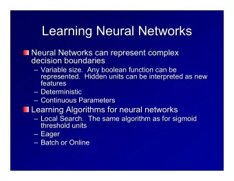
Neural Networks for Machine Learning Lecture 3a Learning the - PowerPoint PPT Presentation

Neural Networks for Machine Learning Lecture 3a Learning the weights of a linear neuron Geoffrey Hinton with Nitish Srivastava Kevin Swersky

Why the perceptron learning procedure cannot be generalised to hidden layers • The perceptron convergence procedure works by ensuring that every time the weights change, they get closer to every “generously feasible” set of weights. – This type of guarantee cannot be extended to more complex networks in which the average of two good solutions may be a bad solution. • So “multi-layer” neural networks do not use the perceptron learning procedure. – They should never have been called multi-layer perceptrons.

A different way to show that a learning procedure makes progress • Instead of showing the weights get closer to a good set of weights, show that the actual output values get closer the target values. – This can be true even for non-convex problems in which there are many quite different sets of weights that work well and averaging two good sets of weights may give a bad set of weights. – It is not true for perceptron learning. • The simplest example is a linear neuron with a squared error measure.

Linear neurons (also called linear filters) weight • The neuron has a real- vector valued output which is a weighted sum of its inputs • The aim of learning is to x i = w T x ∑ y = w i minimize the error summed over all training cases. i input – The error is the squared neuron’s vector difference between the estimate of the desired output and the desired output actual output.

Why don’t we solve it analytically? • It is straight-forward to write down a set of equations, one per training case, and to solve for the best set of weights. – This is the standard engineering approach so why don’t we use it? • Scientific answer: We want a method that real neurons could use. • Engineering answer: We want a method that can be generalized to multi-layer, non-linear neural networks. – The analytic solution relies on it being linear and having a squared error measure. – Iterative methods are usually less efficient but they are much easier to generalize.

A toy example to illustrate the iterative method • Each day you get lunch at the cafeteria. – Your diet consists of fish, chips, and ketchup. – You get several portions of each. • The cashier only tells you the total price of the meal – After several days, you should be able to figure out the price of each portion. • The iterative approach: Start with random guesses for the prices and then adjust them to get a better fit to the observed prices of whole meals.

Solving the equations iteratively • Each meal price gives a linear constraint on the prices of the portions: price = x fish w fish + x chips w chips + x ketchup w ketchup • The prices of the portions are like the weights in of a linear neuron. w = ( w fish , w chips , w ketchup ) • We will start with guesses for the weights and then adjust the guesses slightly to give a better fit to the prices given by the cashier.

The true weights used by the cashier Price of meal = 850 = target linear neuron 150 50 100 2 5 3 portions portions portions of of fish of chips ketchup

A model of the cashier with arbitrary initial weights • Residual error = 350 price of meal = 500 • The “delta-rule” for learning is: Δ w i = ε x i ( t − y ) ε • With a learning rate of 1/35, the weight changes are 50 50 50 +20, +50, +30 • This gives new weights of 2 5 3 70, 100, 80. portions portions portions of – Notice that the weight for of fish of chips ketchup chips got worse!

Deriving the delta rule E = 1 ( t n − y n ) 2 ∑ • Define the error as the squared 2 n ∈ training residuals summed over all training cases: ∂ y n dE n ∂ E = 1 ∑ • Now differentiate to get error dy n 2 ∂ w i ∂ w i derivatives for weights n ( t n − y n ) • The batch delta rule changes n ∑ x i = − the weights in proportion to n their error derivatives summed Δ w i = − ε ∂ E ( t n − y n ) n over all training cases ∑ ε x i = ∂ w i n

Behaviour of the iterative learning procedure • Does the learning procedure eventually get the right answer? – There may be no perfect answer. – By making the learning rate small enough we can get as close as we desire to the best answer. • How quickly do the weights converge to their correct values? – It can be very slow if two input dimensions are highly correlated. If you almost always have the same number of portions of ketchup and chips, it is hard to decide how to divide the price between ketchup and chips.

The relationship between the online delta-rule and the learning rule for perceptrons • In perceptron learning, we increment or decrement the weight vector by the input vector. – But we only change the weights when we make an error. • In the online version of the delta-rule we increment or decrement the weight vector by the input vector scaled by the residual error and the learning rate. – So we have to choose a learning rate. This is annoying.

Neural Networks for Machine Learning Lecture 3b The error surface for a linear neuron Geoffrey Hinton with Nitish Srivastava Kevin Swersky

The error surface in extended weight space • The error surface lies in a space with a horizontal axis for each weight and one E vertical axis for the error. – For a linear neuron with a squared error, it is a quadratic bowl. – Vertical cross-sections are parabolas. – Horizontal cross-sections are w1 ellipses. • For multi-layer, non-linear nets the error surface is much more complicated. w2

Online versus batch learning • The simplest kind of online • The simplest kind of batch learning zig-zags around the learning does steepest descent direction of steepest descent: on the error surface. – This travels perpendicular to constraint from the contour lines. training case 1 w1 w1 constraint from w2 training case 2 w2

Why learning can be slow • If the ellipse is very elongated, the direction of steepest descent is almost w1 perpendicular to the direction towards the minimum! – The red gradient vector has a large w2 component along the short axis of the ellipse and a small component along the long axis of the ellipse. – This is just the opposite of what we want.

Neural Networks for Machine Learning Lecture 3c Learning the weights of a logistic output neuron Geoffrey Hinton with Nitish Srivastava Kevin Swersky

Logistic neurons 1 • These give a real-valued y = ∑ w i z = b + x i output that is a smooth 1 + e − z and bounded function of i their total input. 1 – They have nice 0.5 y derivatives which make learning easy. 0 z 0

The derivatives of a logistic neuron • The derivatives of the logit, z, • The derivative of the output with with respect to the inputs and respect to the logit is simple if the weights are very simple: you express it in terms of the output: ∑ z = b + x i w i 1 y = 1 + e − z i ∂ z ∂ z = x i = w i dy dz = y ( 1 − y ) ∂ w i ∂ x i

The derivatives of a logistic neuron 1 1 + e − z = ( 1 + e − z ) − 1 y = " % dz = − 1 ( − e − z ) e − z " % dy 1 $ ' ' = y (1 − y ) ( 1 + e − z ) 2 = $ ' $ 1 + e − z 1 + e − z # & # & 1 + e − z = (1 + e − z ) − 1 e − z = (1 + e − z ) − 1 1 + e − z = 1 − y because 1 + e − z 1 + e − z

Using the chain rule to get the derivatives needed for learning the weights of a logistic unit • To learn the weights we need the derivative of the output with respect to each weight: ∂ y ∂ z dy dz = x i y (1 − y ) = ∂ w i ∂ w i delta-rule ∂ y n ∂ E ∂ E n y n (1 − y n ) ( t n − y n ) ∑ ∑ x i = = − ∂ y n ∂ w i ∂ w i n n extra term = slope of logistic

Neural Networks for Machine Learning Lecture 3d The backpropagation algorithm Geoffrey Hinton with Nitish Srivastava Kevin Swersky

Learning with hidden units (again) • Networks without hidden units are very limited in the input-output mappings they can model. • Adding a layer of hand-coded features (as in a perceptron) makes them much more powerful but the hard bit is designing the features. – We would like to find good features without requiring insights into the task or repeated trial and error where we guess some features and see how well they work. • We need to automate the loop of designing features for a particular task and seeing how well they work.

Learning by perturbing weights (this idea occurs to everyone who knows about evolution) • Randomly perturb one weight and see if it improves performance. If so, save the change. output units – This is a form of reinforcement learning. – Very inefficient. We need to do multiple forward passes on a representative set hidden units of training cases just to change one weight. Backpropagation is much better. – Towards the end of learning, large input units weight perturbations will nearly always make things worse, because the weights need to have the right relative values.