Sigmoid curves and a case for close-to-linear nonlinear models - PowerPoint PPT Presentation

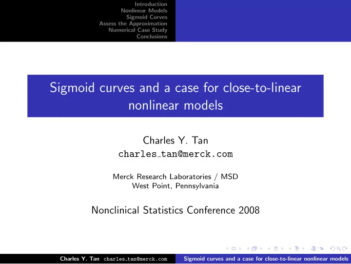
Introduction Nonlinear Models Sigmoid Curves Assess the Approximation Numerical Case Study Conclusions Sigmoid curves and a case for close-to-linear nonlinear models Charles Y. Tan charles tan@merck.com Merck Research Laboratories / MSD West Point, Pennsylvania Nonclinical Statistics Conference 2008 Charles Y. Tan charles tan@merck.com Sigmoid curves and a case for close-to-linear nonlinear models

Introduction Nonlinear Models Sigmoid Curves Assess the Approximation Numerical Case Study Conclusions Outline Introduction Nonlinear Models Sigmoid Curves Assess the Approximation Numerical Case Study Conclusions Charles Y. Tan charles tan@merck.com Sigmoid curves and a case for close-to-linear nonlinear models

Introduction Nonlinear Models Sigmoid Curves Applications and Context Assess the Approximation Statistical Models Numerical Case Study Conclusions Sigmoid curves are common in biological sciences ◮ Quantitative bioanalytical methods ◮ Immunoassays ◮ Bioassays ◮ Hill equation (1910) ◮ Pharmacology ◮ Concentration-effect or dose-response curves ◮ Emax model (1964) ◮ Growth curves ◮ (Population or organ) size as function of time ◮ Mechanistic and empirical ◮ Autocatalytic model (1838, 1908) Charles Y. Tan charles tan@merck.com Sigmoid curves and a case for close-to-linear nonlinear models

Introduction Nonlinear Models Sigmoid Curves Applications and Context Assess the Approximation Statistical Models Numerical Case Study Conclusions Statistics: old favorite and new question ◮ Classic models: (four-parameter) logistic models ◮ Hill equation, Emax model, and autocatalytic model are the same models: logistic models. ◮ They’re symmetric. Charles Y. Tan charles tan@merck.com Sigmoid curves and a case for close-to-linear nonlinear models

Introduction Nonlinear Models Sigmoid Curves Applications and Context Assess the Approximation Statistical Models Numerical Case Study Conclusions Statistics: old favorite and new question ◮ Classic models: (four-parameter) logistic models ◮ Hill equation, Emax model, and autocatalytic model are the same models: logistic models. ◮ They’re symmetric. ◮ New question: what model to use when data are asymmetric ◮ Answer from some quarters: “five-parameter logistic (5PL)” (Richards model) Charles Y. Tan charles tan@merck.com Sigmoid curves and a case for close-to-linear nonlinear models

Introduction Nonlinear Models Sigmoid Curves Applications and Context Assess the Approximation Statistical Models Numerical Case Study Conclusions Statistics: old favorite and new question ◮ Classic models: (four-parameter) logistic models ◮ Hill equation, Emax model, and autocatalytic model are the same models: logistic models. ◮ They’re symmetric. ◮ New question: what model to use when data are asymmetric ◮ Answer from some quarters: “five-parameter logistic (5PL)” (Richards model) ◮ Ratkowsky (1983, 1990): “significant intrinsic curvature”, “a particularly unfortunate model”, “abuse of Occams Razor” ◮ Seber and Wild (1989): “Bad ill-conditioning and convergence problems” Charles Y. Tan charles tan@merck.com Sigmoid curves and a case for close-to-linear nonlinear models

Introduction Nonlinear Models Standard Approach Sigmoid Curves Relative Curvature Assess the Approximation Close-to-Linear Numerical Case Study Conclusions Nonlinear regression y i = f ( x i ; θ ) + ε i , i = 1 , 2 , . . . , n , ◮ Nonlinearity of f with respect to θ : defining characteristics ◮ Nonlinearity of f with respect to x : incidental Charles Y. Tan charles tan@merck.com Sigmoid curves and a case for close-to-linear nonlinear models

Introduction Nonlinear Models Standard Approach Sigmoid Curves Relative Curvature Assess the Approximation Close-to-Linear Numerical Case Study Conclusions Nonlinear regression y i = f ( x i ; θ ) + ε i , i = 1 , 2 , . . . , n , ◮ Nonlinearity of f with respect to θ : defining characteristics ◮ Nonlinearity of f with respect to x : incidental ◮ Homogeneous variance: ε i ’s are i.i.d. N (0 , σ 2 ) Maximum Likelihood = Least Squares Objective function: S ( θ ) = ( y − f ( θ )) ′ ( y − f ( θ )) Charles Y. Tan charles tan@merck.com Sigmoid curves and a case for close-to-linear nonlinear models

Introduction Nonlinear Models Standard Approach Sigmoid Curves Relative Curvature Assess the Approximation Close-to-Linear Numerical Case Study Conclusions 1st order approximation of the model f ( θ ) ≈ f ( θ ∗ ) + F • ( θ − θ ∗ ) , where � ∂ f ( x i ; θ ) � � � F • = F • ( θ ∗ ) = � ∂θ j � θ = θ ∗ n × k Plug it in the definition of S ( θ ), we have a partial 2nd order expansion of S ( θ ) near θ ∗ : S ( θ ) ≈ ε ′ ε − 2 ε ′ F • ( θ − θ ∗ ) + ( θ − θ ∗ ) ′ F ′ • F • ( θ − θ ∗ ) Charles Y. Tan charles tan@merck.com Sigmoid curves and a case for close-to-linear nonlinear models

Introduction Nonlinear Models Standard Approach Sigmoid Curves Relative Curvature Assess the Approximation Close-to-Linear Numerical Case Study Conclusions Common framework for inference S ( θ ∗ ) − S (ˆ θ ) ≈ (ˆ • F • (ˆ • F • ) − 1 F ′ θ − θ ∗ ) ′ F ′ θ − θ ∗ ) ≈ ε ′ F • ( F ′ • ε S (ˆ • F • ) − 1 F ′ θ ) ≈ ε ′ ( I − F • ( F ′ • ) ε Charles Y. Tan charles tan@merck.com Sigmoid curves and a case for close-to-linear nonlinear models

Introduction Nonlinear Models Standard Approach Sigmoid Curves Relative Curvature Assess the Approximation Close-to-Linear Numerical Case Study Conclusions Common framework for inference S ( θ ∗ ) − S (ˆ θ ) ≈ (ˆ • F • (ˆ • F • ) − 1 F ′ θ − θ ∗ ) ′ F ′ θ − θ ∗ ) ≈ ε ′ F • ( F ′ • ε S (ˆ • F • ) − 1 F ′ θ ) ≈ ε ′ ( I − F • ( F ′ • ) ε • F • ) − 1 F ′ Since F • ( F ′ • is idempotent Charles Y. Tan charles tan@merck.com Sigmoid curves and a case for close-to-linear nonlinear models

Introduction Nonlinear Models Standard Approach Sigmoid Curves Relative Curvature Assess the Approximation Close-to-Linear Numerical Case Study Conclusions Common framework for inference S ( θ ∗ ) − S (ˆ θ ) ≈ (ˆ • F • (ˆ • F • ) − 1 F ′ θ − θ ∗ ) ′ F ′ θ − θ ∗ ) ≈ ε ′ F • ( F ′ • ε S (ˆ • F • ) − 1 F ′ θ ) ≈ ε ′ ( I − F • ( F ′ • ) ε • F • ) − 1 F ′ Since F • ( F ′ • is idempotent Local inference: (ˆ • F • (ˆ θ − θ ∗ ) ′ F ′ θ − θ ∗ ) k ∼ n − k F k , n − k S (ˆ θ ) Global inference: S ( θ ∗ ) − S (ˆ θ ) k ∼ n − k F k , n − k S (ˆ θ ) Charles Y. Tan charles tan@merck.com Sigmoid curves and a case for close-to-linear nonlinear models

Introduction Nonlinear Models Standard Approach Sigmoid Curves Relative Curvature Assess the Approximation Close-to-Linear Numerical Case Study Conclusions Intrinsic and parameter-effect curvatures Expectation surface or solution locus: f ( θ ) ∈ R n Its approximation: f ( θ ) ≈ f ( θ ∗ ) + F • ( θ − θ ∗ ) Charles Y. Tan charles tan@merck.com Sigmoid curves and a case for close-to-linear nonlinear models

Introduction Nonlinear Models Standard Approach Sigmoid Curves Relative Curvature Assess the Approximation Close-to-Linear Numerical Case Study Conclusions Intrinsic and parameter-effect curvatures Expectation surface or solution locus: f ( θ ) ∈ R n Its approximation: f ( θ ) ≈ f ( θ ∗ ) + F • ( θ − θ ∗ ) ◮ Planar assumption ◮ The expectation surface is close to its tangent plane. ◮ Intrinsic curvature: deviation at f (ˆ θ ). Charles Y. Tan charles tan@merck.com Sigmoid curves and a case for close-to-linear nonlinear models

Introduction Nonlinear Models Standard Approach Sigmoid Curves Relative Curvature Assess the Approximation Close-to-Linear Numerical Case Study Conclusions Intrinsic and parameter-effect curvatures Expectation surface or solution locus: f ( θ ) ∈ R n Its approximation: f ( θ ) ≈ f ( θ ∗ ) + F • ( θ − θ ∗ ) ◮ Planar assumption ◮ The expectation surface is close to its tangent plane. ◮ Intrinsic curvature: deviation at f (ˆ θ ). ◮ Uniform-coordinate assumption ◮ Straight parallel equispaced lines in the parameter space R k map into straight parallel equispaced lines in the expectation surface (as they do in the tangent plane). ◮ Parameter-effect curvature: deviation at f (ˆ θ ). Charles Y. Tan charles tan@merck.com Sigmoid curves and a case for close-to-linear nonlinear models

Introduction Nonlinear Models Standard Approach Sigmoid Curves Relative Curvature Assess the Approximation Close-to-Linear Numerical Case Study Conclusions Curvatures (nonlinearity) are local properties ◮ The model f ◮ The parameters θ ◮ Parameterization ◮ Values ◮ The design x ◮ Sample size ◮ Values ◮ The particular realization of ε Charles Y. Tan charles tan@merck.com Sigmoid curves and a case for close-to-linear nonlinear models