Pooling versus model selection for nowcasting with many predictors: - PowerPoint PPT Presentation
Pooling versus model selection for nowcasting with many predictors: An application to German GDP Vladimir Kuzin Massimiliano Marcellino DIW Berlin EUI Florence Christian Schumacher Deutsche Bundesbank 1 Introduction 1.1 What is
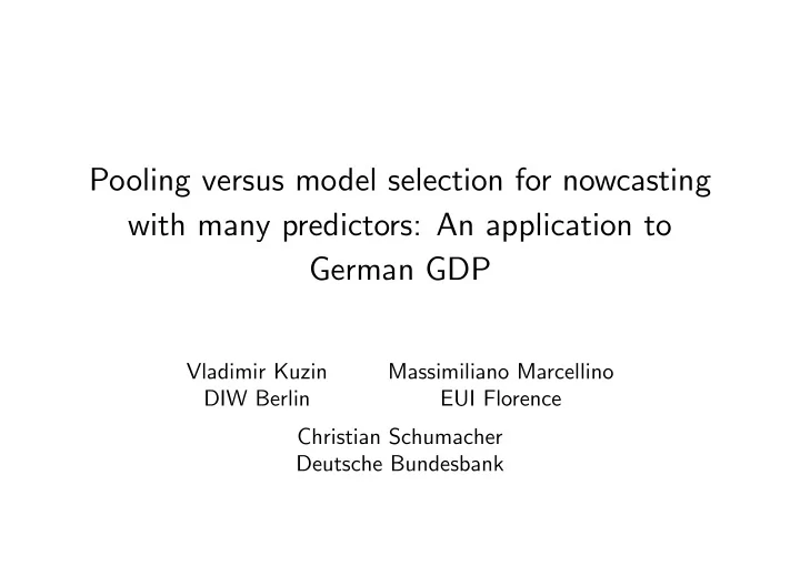
Pooling versus model selection for nowcasting with many predictors: An application to German GDP Vladimir Kuzin Massimiliano Marcellino DIW Berlin EUI Florence Christian Schumacher Deutsche Bundesbank
1 Introduction 1.1 What is nowcasting? decision makers regularly request information on the current state of the economy, in particular with respect to GDP GDP is a comprehensive business cycle indicator, but sampled at quarterly fre- quency only and published with considerable delay example: at the beginning of May, German GDP is available only for the fourth quarter of the previous year; to obtain a 2 nd quarter GDP nowcast, we have to make a projection with forecast horizon of two quarters from the end of the GDP sample economist’s task: estimate current quarter GDP using all information which is currently available
1.2 Why is nowcasting GDP challenging? there are many difficulties, we discuss two, both leading to unbalanced data : 1. GDP is quarterly data, many important indicators are sampled at monthly or higher frequency - mixed-frequency problem 2. indicators for nowcasting are available with different publication lags → leads to the so-called ragged edge of multivariate datasets, Wallis (1986) question here: how to nowcast quarterly German GDP with a large set of monthly indicators with missing observations?
1.3 Nowcast approaches from the recent literature 1. mixed-data sampling or MIDAS regressions with a few predictors , see Ghysels, Sinko, and Valkanov (2007) EctrRev, Clements and Galvão (2009) JBES 2. factor models based on large datasets: (a) large state-space factor model by Giannone, Reichlin, and Small (2008) JME (b) New Eurocoin based on dynamic principal components, Altissimo et al. (2007) CEPR WP - used by CEPR to assess the current state of the economy 3. a mix of both: Factor-MIDAS , Marcellino and Schumacher (2010) OBES: fac- tors are estimated on ragged-edge data and plugged into MIDAS regressions
1.4 Pooling versus model selection in empirical forecast exercises of the model developers, all the single approaches above performed well we also evaluate the performance of pooling of forecasts from these models why pooling? stylised fact from forecast literature: very good forecast performance of pooling, Timmermann (2005) HdBEcForec why pooling? specifying or selecting single nowcast models can be difficult within each model class above, we have to make a lot of decisions concerning specification : variable selection, factor estimation method, number of factors, au- toregressive dynamics → potential misspecification
in theory, pooling provides insurance against misspecification of single models and structural breaks, Clements and Hendry (2004) EctrcsJ recent empirical evidence that supports pooling based on balanced data: Clark and McCracken (2010) JAE fc, Assenmacher-Wesche and Pesaran (2008) NIEcRev
1.5 What we do we provide an empirical comparison exercise of nowcast pooling for German GDP based on about one hundred monthly predictors with a ragged edge we compare pooling to model selection of single models , where alternative model selection procedures are applied, e.g. information criteria, past performance outline: 2. MIDAS regressions 3. Factor-MIDAS with factors estimated from many indicators 4. Empirical now- and forecast comparison 5. Conclusions
2 MIDAS regressions Ghysels, Sinko, Valkanov (2007) EctrRev, Clements and Galvão (2009) JBES MIDAS equation for quarterly GDP growth y t q + h q and forecast horizon h q explained by one particular monthly indicator x t m y t q + h q = β 0 + β 1 b ( L m , θ ) x (3) t m + ε t q + h q (1) K exp( θ 1 k + θ 2 k 2 ) � c ( k, θ ) L k b ( L m , θ ) = c ( k, θ ) = (2) m K � k =0 exp( θ 1 k + θ 2 k 2 ) k =0 with L m x t m = x t m − 1 and time indices are related by t q = t m / 3 superscript in x (3) t m indicates that sampling frequency of x t m is three times higher than for y t q
2.1 Dynamics GDP is explained by monthly indicator and its monthly lags x (3) t m − i i = 0 , 1 , . . . , K with unrestricted b ( L m ) , large K leads to overparameterized model to solve this, lag polynomial is non-linear exponential (Almon) determined by two coefficents θ 1 , θ 2 only, to be estimated by nonlinear least squares (NLS) for large lag orders and mixing of data with very different frequencies, MIDAS is parametrically very parsimonious
2.2 Forecasting MIDAS equation is based on direct estimation technique, see Marcellino, Stock, Watson (2006) JEctrcs: LHS variables are t q + h q -dated, whereas RHS predictors are t m -dated for each horizon h q = h m / 3 , we have a different model: β 1 b ( L m , � y T q + h q | T m = � β 0 + � θ ) x T m (3) Note: For estimation, we have to use skip-sampled x (3) t m , whereas MIDAS exploits all monthly (lagged) observations x T m , x T m − 1 , ..., in the forecast by b ( L m , � θ ) x T m
2.3 Additional MIDAS features MIDAS regressions take into account the the most recent observations of the indicator , which is often more timely available than GDP MIDAS can be augmented by autoregressive terms , taking into account potential hikes in the IRF, Clements and Galvão (2009) JBES more than one predictor can be taken into account simply by adding terms to the regression: per predictor x j,t m , the number of coefficients increases by three ( β 1 ,j , θ 1 ,j , θ 2 ,j ) however, in the application below, we forecast with MIDAS and one indicator only, taken from a large set of potential predictors (single-indicator MIDAS)
3 Factor-MIDAS with factors estimated from many indicators Marcellino and Schumacher (2010) OBES: Factor-MIDAS based on mixed-frequency and ragged-edge data is a two-step procedure , see Boivin and Ng (2005) IJCB for the single-frequency case 1. estimate factors based on monthly ragged-edge data 2. make a nowcast with MIDAS, where factor estimates are the predictors
3.1 Some simple theory behind Factor-MIDAS Marcellino and Schumacher (2008) CEPR WP, revised: monthly one-factor ( r = 1 ) model X t m = Λ f t m + ξ t m (4) and assume that monthly unobserved GDP growth is part of X t m , y t m ∈ X t m y t m = λ y f t m + ξ y,t m (5) assume AR model for the factor and idiosyncratic components f t m = ρ f f t m + e f,t m (6) ξ y,t m = ρ ξ y ξ y,t m − 1 + e ξ y ,t m (7) given this monthly factor specification, we can write the factor representation for y three months ahead y t m +3 = κ 0 y t m + κ 1 f t m + κ e f ( L m ) e f,t m +3 + κ ξ y ( L m ) e ξ y ,t m +3 (8)
consider time aggregation y t q = (1 + 2 L m + 3 L 2 m + 2 L 3 m + L 4 m ) y t m = ϕ y ( L m ) y t m for t m = 3 , 6 , 9 , ... and t m = 3 t q , and multiply by ϕ y ( L m ) on both sides of the equation (1 − κ 0 L 3 m ) ϕ y ( L m ) y t m +3 = κ 1 ϕ y ( L m ) f t m + ϕ y ( L m )( κ e f ( L m ) e f,t m +3 + κ ξ y ( L m ) e ξ y ,t m +3 ) (9) as time aggregation implies y t q +1 = ϕ y ( L m ) y t m +3 , this is like a MIDAS equation with parameter restrictions from the factor model and the time aggregation scheme Factor-MIDAS should be regarded as an approximation rather than a structural model the residual in MIDAS can be serially dependent , which is typical for direct estimation
3.2 Factor estimation with ragged-edge data assumption: monthly ( N × 1) vector X t m with N large has a factor structure X t m = ΛF t m + ξ t m (10) with factors F t m = ( f 1 ,t m , . . . , f r,t m ) � , loadings Λ , idiosyncratic components ξ t m if data X = ( X 1 , . . . , X T m ) � is balanced, there are different ways to estimate F : principal components analysis (PCA) as in Stock and Watson (2002) JBES; dy- namic PCA as in Forni et al. (2005) JASA; subspace algorithms, Marcellino and Kapetanios (2009) JTSA this ’first wave’ of factor forecast papers does not consider the difficulties of real-time data (ragged edge, mixed frequencies)
3.2.1 Vertical realignment of the data and dynamic PCA same procedure as in New Eurocoin , Altissimo et al. (2006) CEPR WP variable i is released with k i months of publication lag → in period T m , the final observation available is in period T m − k i balancing by ‘vertical’ realignment x i,T m = x i,T m − k i � (11) applying this procedure for each series and harmonising at the beginning of the sample yields a balanced data set � X t m factor estimation from � X t m by Dynamic PCA , Forni et al. (2005) JASA
3.2.2 Kalman smoother estimation in a large state-space model Doz, Giannone and Reichlin (2006) ECB WP, Giannone, Reichlin and Small (2008) JME: X t m = ΛF t m + ξ t m (12) Ψ( L m ) F t m = B η t m (13) factor VAR with Ψ( L m ) = � p i =1 Ψ i L i m and L m x t m = x t m − 1 , q -dimensional vector η t m contains dynamic shocks that drive factors, identification matrix B is ( r × q )- dimensional model has state-space representation with factors as states, Kalman smoother pro- vides factor estimates given the coefficients coefficients are estimated outside state-space model based on initial PCA factors, no iterative ML, rather 2-step
4 Empirical nowcast comparison 4.1 Data and nowcast simulation design data: German quarterly GDP from 1992 Q 1 until 2007 Q 4 , 111 monthly indicators recursive design with increasing sample size: each month, we re-estimate models and compute new nowcasts with monthly horizon h m = 1 , 2 , . . . , 6 evaluation sample from 2000 Q 1 until 2007 Q 4 statistic: MSE relative to in-sample mean naive forecast
4.2 Empirical results
Recommend
More recommend
Explore More Topics
Stay informed with curated content and fresh updates.
