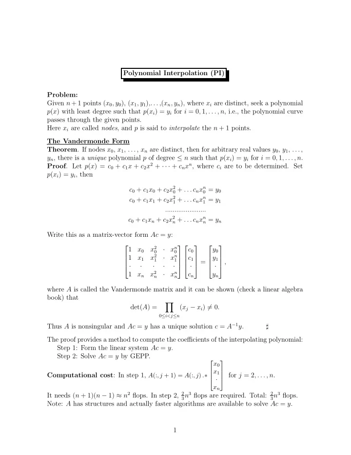
Polynomial Interpolation (PI) Problem: Given n + 1 points ( x 0 , y - PDF document

Polynomial Interpolation (PI) Problem: Given n + 1 points ( x 0 , y 0 ), ( x 1 , y 1 ),. . . ,( x n , y n ), where x i are distinct, seek a polynomial p ( x ) with least degree such that p ( x i ) = y i for i = 0 , 1 , . . . , n , i.e., the polynomial curve passes through the given points. Here x i are called nodes , and p is said to interpolate the n + 1 points. The Vandermonde Form Theorem . If nodes x 0 , x 1 , . . . , x n are distinct, then for arbitrary real values y 0 , y 1 , . . . , y n , there is a unique polynomial p of degree ≤ n such that p ( x i ) = y i for i = 0 , 1 , . . . , n . Proof . Let p ( x ) = c 0 + c 1 x + c 2 x 2 + · · · + c n x n , where c i are to be determined. Set p ( x i ) = y i , then c 0 + c 1 x 0 + c 2 x 2 0 + . . . c n x n 0 = y 0 c 0 + c 1 x 1 + c 2 x 2 1 + . . . c n x n 1 = y 1 ...................... c 0 + c 1 x n + c 2 x 2 n + . . . c n x n n = y n Write this as a matrix-vector form Ac = y :  x 2 x n      1 x 0 · c 0 y 0 0 0 x 2 x n 1 x 1 · c 1 y 1       1 1  =  ,       · · · · · · ·     x 2 x n 1 x n · c n y n n n where A is called the Vandermonde matrix and it can be shown (check a linear algebra book) that � det( A ) = ( x j − x i ) � = 0 . 0 ≤ i<j ≤ n Thus A is nonsingular and Ac = y has a unique solution c = A − 1 y . ♯ The proof provides a method to compute the coefficients of the interpolating polynomial: Step 1: Form the linear system Ac = y . Step 2: Solve Ac = y by GEPP.  x 0  x 1 Computational cost : In step 1, A (: , j + 1) = A (: , j ) . ∗    for j = 2 , . . . , n .   ·  x n It needs ( n + 1)( n − 1) ≈ n 2 flops. In step 2, 2 3 n 3 flops are required. Total: 3 n 3 flops. 2 Note: A has structures and actually faster algorithms are available to solve Ac = y . 1

Evaluating p ( x ): Nested multiplication c 0 + c 1 x + c 2 x 2 + . . . c n x n p ( x ) = = c 0 + x ( c 1 + x ( c 2 + . . . + x ( c n − 1 + xc n )) · · · ) . Procedure for evaluating p ( x ) for some x : p ← c n for i = n − 1 : − 1 : 0 p ← c i + xp end Computational cost : 2 n flops. The Lagrange Form Lagrange form (LF): n � p ( x ) = l i ( x ) y i , i =0 where � 0 , ( x − x 0 ) · · · ( x − x i − 1 )( x − x i +1 ) · · · ( x − x n ) i � = j l i ( x ) = ( x i − x 0 ) · · · ( x i − x i − 1 )( x i − x i +1 ) · · · ( x i − x n ) , l i ( x j ) = 1 , i = j Obviously p ( x ) defined above is a polynomial of degree less than or equal to n and p ( x i ) = y i for i = 0 , 1 , . . . , n . We can rewrite p ( x ): n n n j =0 ,j � = i ( x i − x j ) · Π n j =0 ( x − x j ) y i c i � � � p ( x ) = l i ( x ) y i = = q ( x ) Π n x − x i x − x i i =0 i =0 i =0 y i where c i ≡ j =0 ,j � = i ( x i − x j ) , q ( x ) ≡ Π n j =0 ( x − x j ). Π n Computational cost of finding c 0 , c 1 , . . . , c n : For each i , computing c i needs 1 division, n subtractions, n − 1 multiciplations, a total of 2 n flops. So computing all c i needs 2 n ∗ ( n + 1) ≈ 2 n 2 flops. Computational cost of evaluating p ( x ) for some x (given c i for i = 0 , . . . , n ): c i Computing q ( x ) needs 2 n + 1 flops. Computing x − x i needs 2 flops for each i . Thus computing p ( x ) needs a total of (2 n + 1) + ( n + 1) ∗ 2 + n ≈ 5 n flops. Note: In practice we usually do not use the Lagrange form, since the evaluation of p ( x ) is not efficient. 2

The Newton Form Idea: Suppose a polynomial p k ( x ) of degree ≤ k has been found to interpolate ( x 0 , y 0 ), ( x 1 , y 1 ),. . . ,( x k , y k ). We seek a polynomial p k +1 ( x ) of degree ≤ k + 1 to interpolate ( x 0 , y 0 ), ( x 1 , y 1 ),. . . , ( x k , y k ), ( x k +1 , y k +1 ). Let p k +1 ( x ) = p k ( x ) + a k +1 ( x − x 0 )( x − x 1 ) . . . ( x − x k ), where a k +1 is to be determined. Obviously we have p k +1 ( x i ) = p k ( x i ) = y i , 0 ≤ i ≤ k. Set p k +1 ( x k +1 ) = y k +1 , we obtain y k +1 − p k ( x k +1 ) a k +1 = ( x k +1 − x 0 )( x k +1 − x 1 ) · · · ( x k +1 − x k ) . This p k +1 ( x ) with the above a k +1 interpolates ( x 0 , y 0 ) , . . . , ( x k +1 , y k +1 ). Also notice p k +1 ( x ) is a polynomial of degree ≤ k + 1. So it is what we seek. Finally p n has the so-called Newton form (NF): p n ( x ) = a 0 + a 1 ( x − x 0 ) + a 2 ( x − x 0 )( x − x 1 ) + . . . + a n ( x − x 0 )( x − x 1 ) · · · ( x − x n − 1 ) . Evaluating p n ( x ) for some x : Nested multiplication p n ( x ) = a 0 + a 1 ( x − x 0 ) + a 2 ( x − x 0 )( x − x 1 ) + . . . + a n ( x − x 0 )( x − x 1 ) · · · ( x − x n − 1 ) = ( · · · (( a n ( x − x n − 1 ) + a n − 1 )( x − x n − 2 ) + a n − 2 ) · · · )( x − x 0 ) + a 0 Procedure for evaluating p n ( x ): p ← a n for i = n − 1 : − 1 : 0 p ← p ∗ ( x − x i ) + a i end Computational cost of this procedure : 3 n flops. Cost of computing a 1 , a 2 , . . . a n by y k +1 − p k ( x k +1 ) a k +1 = ( x k +1 − x 0 )( x k +1 − x 1 ) · · · ( x k +1 − x k ) : Cost of computing a k +1 : (1 + 3 k ) + [( k + 1) + k ] + 1 = 5 k + 3 flops. 2 n 2 + 1 2 n 2 flops. Total cost: � n − 1 k =0 (5 k + 3) = 5 2 n ≈ 5 3

A more efficient method for computing a 0 , a 1 , . . . , a n Since n i − 1 � � p n ( x ) = a i ( x − x j ) i =0 j =0 interpolates ( x i , y i ) for i = 0 , 1 . . . , n , we have p n ( x i ) = y i , i = 0 , 1 . . ., n. This gives the linear system Aa = y : 1   1 x 1 − x 0    a 0   y 0  1    �  a 1 y 1 1 x 2 − x 0 ( x 2 − x j )             a 2 = y 2 . j =0             · · · · · ·         1 n − 1 a n y n   � � 1 x n − x 0 ( x n − x j ) · ( x n − x j )   j =0 j =0 Notice A is a lower triangular matrix and its diagonal elements are nonzero, so A is nonsingular and Aa = y has a unique solution a = A − 1 y . Since A has special structure, we can design an efficient algorithm to compute the solution a . The pattern of finding a 0 , a 1 , . . . , a n : for k = 0 : n − 1 a k ← y k (updated y k ) for i = k + 1 : n subtract equation k from equation i and divide equation i by x i − x k end end a n ← y n Notice when we update the equations we need only keep track of changes in the y vector. Algorithm . Given x i , y i , find a i ( i = 0 , . . . , n ): for k = 0 : n − 1 a k ← y k for i = k + 1 : n y i ← ( y i − y k ) / ( x i − x k ) end end a n ← y n 4

Remark: The computation can be performed in a table (an example will be given in class). 2 n 2 flops. Computational cost : � n − 1 k =0 3( n − k ) = 3 2 n ( n + 1) ≈ 3 Dangers of High Degree Polynomial Interpolation Let y = f ( x ). We approximate f on [ a, b ] by an interpolating polynomial p at n + 1 nodes, i.e., p ( x i ) = y i = f ( x i ) . Q . Is it true that f will be well approximate at all intermediate points as the number of nodes increases? Answer: No. The Runge function: f ( x ) = 1 / (1 + 25 x 2 ) , x ∈ [ − 1 , 1] . If p n is the polynomial that interpolates the f at n + 1 equally spaced points on [ − 1 , 1], then n →∞ max lim − 1 ≤ x ≤ 1 | f ( x ) − p n ( x ) | = ∞ . We could choose better nodes. But in general high-degree polynomial interpolation should be avoided. Interpolation error theorem : If p is the polynomial of degree at most n that inter- polates f at the n + 1 distinct nodes x 0 , x 1 , . . . , x n belonging to [ a, b ] and if f ( n +1) is continuous. Then for any x in [ a, b ], there is z x in ( a, b ) for which 1 ( n + 1)! f ( n +1) ( z x ) Π n f ( x ) − p ( x ) = i =0 ( x − x i ) . 5