Cubic spline interpolation High-degree polynomial fitting has strong - PowerPoint PPT Presentation
Cubic spline interpolation High-degree polynomial fitting has strong oscillations. Can we get a piecewise low degree polynomial interpolation instead? S ( x ) S n 2 S n 1 S j S 1 S j 1 S 0 S j ( x j 1 ) f ( x j 1 )
Cubic spline interpolation High-degree polynomial fitting has strong oscillations. Can we get a piecewise “low degree” polynomial interpolation instead? S ( x ) S n � 2 S n � 1 S j S 1 S j � 1 S 0 S j ( x j � 1 ) � f ( x j � 1 ) � S j � 1 ( x j � 1 ) S j ( x j � 1 ) � S j � 1 ( x j � 1 ) � � S j ( x j � 1 ) � S j � 1 ( x j � 1 ) � � x x 0 x 1 x 2 x j x j � 1 x j � 2 x n � 2 x n � 1 x n . . . . . . Numerical Analysis I – Xiaojing Ye, Math & Stat, Georgia State University 122
Cubic spline interpolation Suppose we are given x 0 , . . . , x n and f ( x i ), ∀ i , we want to find a cubic spline interpolation S ( x ), s.t. 1. S ( x ) is a cubic polynomial, denoted by S j ( x ), on [ x j , x j +1 ]; 2. S j ( x j ) = f ( x j ), S j ( x j +1 ) = f ( x j +1 ) 3. S j ( x j ) = S j +1 ( x j ) for all j (consequence of Item 2.) 4. S ′ j +1 ( x j +1 ) = S ′ j ( x j +1 ) for all j 5. S ′′ j +1 ( x j +1 ) = S ′′ j ( x j +1 ) for all j 6. One of the following boundary condition is satisfied: ◮ S ′′ ( x 0 ) = S ′′ ( x n ) = 0 (natural/free boundary condition) ◮ S ′ ( x 0 ) = f ′ ( x 0 ) and S ′ ( x n ) = f ′ ( x n ) (clamped boundary condition) Numerical Analysis I – Xiaojing Ye, Math & Stat, Georgia State University 123
Cubic spline interpolation Remarks 1. S ( x ) only agrees with f ( x ) at x i , not necessarily f ′ ( x ). 2. Clamped BC is more accurate than natural BC, but needs f ′ ( a ) , f ′ ( b ). Numerical Analysis I – Xiaojing Ye, Math & Stat, Georgia State University 124
Example Example (Construct a natural cubic spline) Construct natural cubic spline for f ( x ) = e x using x i = i for i = 0 , 1 , 2 , 3. y e 3 y = S ( x ) y = e x e 2 e 1 x 1 2 3 Numerical Analysis I – Xiaojing Ye, Math & Stat, Georgia State University 125
Construction of cubic splines Given { ( x i , f ( x i )) : i = 0 , . . . , n } , we need to construct n cubic polynomials, each with 4 coefficients S j ( x ) = a j + b j ( x − x j ) + c j ( x − x j ) 2 + d j ( x − x j ) 3 on [ x j , x j +1 ] , ∀ j So we have 4 n unknowns to determine: a j , b j , c j , d j , for j = 0 , . . . , n − 1 Numerical Analysis I – Xiaojing Ye, Math & Stat, Georgia State University 126
Construction of cubic splines The cubic spline conditions will determine these 4 n coefficients uniquely ( h j := x j +1 − x j ) according to the 6 rules: 1. By definition of S j . 2. Since S j ( x j ) = a j = f ( x j ), we get a j for j = 0 , . . . , n − 1. 3. a j +1 = S j +1 ( x j +1 ) = S j ( x j +1 ) = a j + b j h j + c j h 2 j + d j h 3 j . j ( x ) = b j + 2 c j ( x − x j ) + 3 d j ( x − x j ) 2 , therefore S ′ 4. S ′ j ( x j ) = b j j ( x j +1 ) = b j + 2 c j h j + 3 d j h 2 and b j +1 = S ′ j +1 ( x j +1 ) = S ′ j . 5. S ′′ j ( x ) = 2 c j + 6 d j ( x − x j ). Then we have S ′′ j ( x j ) = 2 c j . So 2 c j +1 = S ′′ j +1 ( x j +1 ) = S ′′ j ( x j ) = 2 c j + 6 d j h j . 6. Use the required boundary condition. ◮ Natural BC: c 0 = c n = 0 ◮ Clamped BC: b 0 = f ′ ( a ), b n = f ′ ( b ). Numerical Analysis I – Xiaojing Ye, Math & Stat, Georgia State University 127
Construction of cubic splines As we have known the values of a j , we can combine equations from the last 3 items to solve for c j and obtain h j − 1 c j − 1 +2( h j − 1 + h j ) c j + h j c j +1 = 3 3 ( a j +1 − a j ) − ( a j − a j − 1 ) h j h j − 1 for each j = 1 , . . . , n − 1. If we assume natural splines with S ′′ 0 ( x 0 ) = S ′′ n − 1 ( x n ) = 0, then c 0 = c n = 0. Numerical Analysis I – Xiaojing Ye, Math & Stat, Georgia State University 128
Recommend
More recommend
Explore More Topics
Stay informed with curated content and fresh updates.









![1 Example Evaluating Bzier and B-Spline Curves, t in [0,1] f(0,0,0) f(0,0,1) f(0,1,1)](https://c.sambuz.com/1006742/1-s.webp)
