Poisson Image Editing and opaque source image regions into a - PDF document

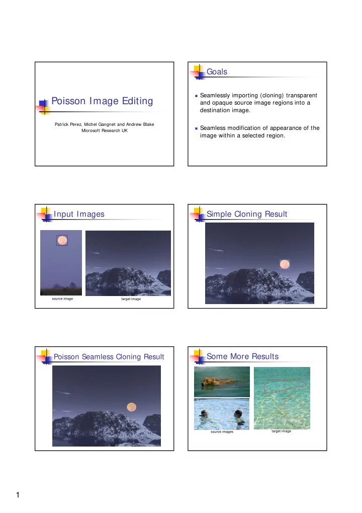
Goals � Seamlessly importing (cloning) transparent Poisson Image Editing and opaque source image regions into a destination image. Patrick Perez, Michel Gangnet and Andrew Blake � Seamless modification of appearance of the Microsoft Research UK image within a selected region. Input Images Simple Cloning Result source image target image Some More Results Poisson Seamless Cloning Result target image source images 1

Some More Results Some More Results simple cloning Poisson seamless cloning source images source images Interpolation Membrane Interpolant � Solve the following minimization problem: min ∫∫ 2 ∇ f f Ω • S: a closed subset of R 2 � subject to Dirichlet boundary conditions: • Ω : a closed subset of S, with boundary ∂Ω ∂ = * f f • f* : known scalar function over S\ Ω Ω ∂ Ω • f: unknown scalar function over Ω Euler-Lagrange Equation Euler-Lagrange (continued) ( ) = ∇ = + 2 2 2 F f f f � A fundamental equation of calculus of variations , � In our case: x y which states that if J is defined by an integral of ∂ ∂ ∂ the form: ∫ = F d F d F − − = J F ( x , f , f x ) dx � The equation is: 0 ∂ ∂ ∂ f dx f dy f x y ∂ ∂ ∂ 2 d F d f � then J has a stationary value if the following F = = = and 2 f 2 0 � ∂ ∂ ∂ x differential equation is satisfied: 2 f dx f dx x x ∂ ∂ F d F − = ∂ ∂ 2 2 0 � So we get: f f + = Δ = ∂ ∂ f dx f f 0 x ∂ ∂ 2 2 x y 2

Smooth Image Completion Discrete Approximation Δ = Ω ∂ = * f 0 over s . t . f f Euler-Lagrange: Ω ∂ Ω ∂ ∂ 2 2 f f Δ = + ∫∫ f ∇ 2 = arg min * ∂ ∂ 2 2 f s . t . f f x y ∂ Ω ∂ Ω Ω f ∂ ∂ f 2 ≅ 1 − f f f ≅ − + + f 2 f f ∂ The minimum is achieved when: x , y x , y + − x ∂ x 1 , y x , y x 1 , y 2 x Δ ≅ − + + − + = Δ = Ω ∂ = f x y ( , ) f 2 f f f 2 f f * f 0 over s . t . f f + − + − x 1, y x y , x 1, y x y , 1 x y , x y , 1 Ω ∂ Ω = + + + + − = f f f f 4 f 0 + − + − x 1, y x 1, y x y , 1 x y , 1 x y , Wow result Solving � Each f x,y is an unknown variable x i , total of N variables (covering the unknown pixels) f x,y-1 +f x-1,y -4f x,y +f x+1,y +f x,y+1 =0 or x i-w +x i-1 -4x i +x i+1 +x i+w =0 � Reduces to the sparse algebraic system: x 1 0 1 1 -4 1 1 ground truth input result x 2 0 Known values of f() … b 1 1 1 -4 1 1 contribute to the left side b 2 x i-w +x i-1 -4x i +x i+1 =-f(x,y+1) 1 1 -4 1 1 = 0 0 0 x N b 3 0 N x N Guided Interpolation Poisson Cloning: “Guiding” the completion � Laplace equation yields a smooth interpolant. � Idea: use a guiding vector field v . � We can guide the completion to fill the hole using gradients from another source image � Reverse: Seek a function f whose gradients are closest to the gradients of the source image 3

Guided Interpolant Poisson Equation � Solve the following minimization problem: � This time the Euler-Lagrange equation reduces to the Poisson equation: 2 ∫∫ ∇ − min f G ∂ ∂ ∂ ∂ 2 2 G f f G + = + f y x Ω ∂ ∂ ∂ ∂ 2 2 x y x y � written more concisely as: � subject to Dirichlet boundary conditions: ∂ = * f f Δ = f div G Ω ∂ Ω Poisson Cloning Poisson Cloning (Solving) Each f x,y is a variable x i as before, solving = ∇ G source image Denote ∫∫ ∇ − 2 = f x,y-1 +f x-1,y -4f x,y +f x+1,y +f x,y+1 =divG(x,y) arg min * f G s . t . f f ∂ Ω ∂ Ω Ω f Or Δ = Ω ∂ = * f div G over s . t . f f Ω ∂ Ω x i-w +x i-1 -4x i +x i+1 +x i+w =divG(x,y) (backward difference) ∂ ∂ As before it reduces to a sparse algebraic system G G = + ≅ − − + − − div G G ( x , y ) G ( x 1 , y ) G ( x , y ) G ( x , y 1 ) x x y y dx dy Seamless Cloning Concealment � Choose the gradient field of the source image as the guiding vector field G . 4

Insertion Feature Exchange Texture Swapping Mixing Gradients � Sometimes it is desirable to define the guiding field as a mixture of source and target gradient fields. � Option A: linear combination of the gradient fields � Option B: strongest gradient wins: ⎧ ∇ ∇ > ∇ * * f ( ) if f ( ) g ( ) x x x = ⎨ ( ) v x ∇ ⎩ g ( ) otherwise x 5

More Mixtures More Mixtures Selection Editing Local Illumination Changes � Texture flattening: use target gradient field only where edges are detected: = ∇ * x ( ) M ( ) f ( ) v x x Local Color Changes Seamless Tiling 6