Point processes characterized by their one dimensional distributions - PowerPoint PPT Presentation
Point processes characterized by their one dimensional distributions Aihua Xia Department of Mathematics and Statistics The University of Melbourne, VIC 3010 8 July 2013 [Slide 1] Independence and uncorrelation For a bivariate random vector (
Point processes characterized by their one dimensional distributions Aihua Xia Department of Mathematics and Statistics The University of Melbourne, VIC 3010 8 July 2013 [Slide 1]
Independence and uncorrelation For a bivariate random vector ( X, Y ) with finite second moments, we can define Cov( X, Y ) = E [( X − E X )( Y − E Y )] and its joint joint cdf F X,Y ( x, y ) = P ( X ≤ x, Y ≤ y ). • X and Y are uncorrelated if Cov( X, Y ) = 0 • X and Y are indept if F X,Y ( x, y ) = F X ( x ) F Y ( y ) for all x and y • If X and Y are independent, then they are uncorrelated. • When does uncorrelation imply independence? [Slide 2]
Independence and uncorrelation (2) • If X and Y takes two values? X 0 1 Y 0 p 00 p 01 1 p 10 p 11 E ( XY ) = p 11 , E X = p 01 + p 11 =: p · 1 and E Y = p 10 + p 11 =: p 1 · , so Cov( X, Y ) = 0 iff p 11 = p · 1 p 1 · iff X and Y are indept. [Slide 3]
In general, X a 0 a 1 Y b 0 p 00 p 01 b 1 p 10 p 11 X and Y are indept iff they are uncorrelated. • One takes two values and the other takes more than two? [Slide 4]
Reformulation • Given that F is an n -dimensional df and G an m dimensional df, a coupling of F and G is a random vector ( X 1 , . . . , X n ; Y 1 , . . . , Y m ) such that ( X 1 , . . . , X n ) ∼ F and ( Y 1 , . . . , Y m ) ∼ G . • Assume that both F and G have finite second moments, what are the conditions such that any uncorrelated coupling must be an independent coupling? [Slide 5]
Rank We say that F has rank k if its support is k -dimension. He and X. (1987): if F has rank k and G has rank l , then any uncorrelated coupling is an independent coupling iff F has at most k + 1 points and G has at most l + 1 values. [Slide 6]
In the context of processes Viewing ( X 1 , . . . , X n ; Y 1 , . . . , Y m ) as a process on { 1 , 2 , . . . , n + m } , the problem becomes How to specify the distribution of a process from its marginal distributions plus something else? [Slide 7]
What’s something else? Example. X = ( I 1 , I 2 ) =: I 1 δ 1 + I 2 δ 2 with I 1 , I 2 two indicator rv’s and assume we know P ( I 1 = 0), P ( I 2 = 0) and P ( I 1 + I 2 = 0) (abstraction: avoidance function ), then P ( I 1 = 0 , I 2 = 0) = P ( I 1 + I 2 = 0) , P ( I 1 = 0 , I 2 = 1) = P ( I 1 = 0) − P ( I 1 = 0 , I 2 = 0) , P ( I 2 = 0) − P ( I 1 = 0 , I 2 = 0) , P ( I 1 = 1 , I 2 = 0) = P ( I 1 = 1 , I 2 = 1) = easy . [Slide 8]
Remark • Cov( I 1 , I 2 ) = 0 specifies P ( I 1 = 1 , I 2 = 1) • avoidance function specifies P ( I 1 = 0 , I 2 = 0) [Slide 9]
Generally If I 1 , . . . , I k are indicator rv’s, then the distribution of ( I 1 , I 2 , . . . , I k ) is uniquely determined by the probabilities of P ( I i 1 + · · · + I i l = 0) for all 1 ≤ l ≤ k and 1 ≤ i 1 < i 2 < · · · < i l ≤ k . Proof. By math induction on k . [Slide 10]
Why not point processes? • Γ is a metric space, typically R + , R or R d • We define H as the class of all integer-valued locally finite measures on H equipped with a σ -field • Ξ is a measurable mapping from a probability space to H and is called a point process • A point process Ξ is called simple if, almost surely, Ξ( ω ) takes either 1 point or no points at each location. • The previous example is a simple point process [Slide 11]
The complete distribution of a PP [Kallenberg (1983) or Daley and Vere-Jones (1988)] To specify the complete distribution of a point process Ξ, it is necessary and sufficient to specify all finite distributions (Ξ( B 1 ) , ..., Ξ( B k )) for all k ≥ 1 and all disjoint Borel sets B 1 , ..., B k . [Slide 12]
Simple point processes Renyi (1967) and M¨ onch (1971): the distribution of a simple point process is determined by the probability of there being 0 points (avoidance function) in each of the Borel sets. [Slide 13]
Example A simple point process Ξ is a Poisson process on Γ iff for any Borel B ⊆ Γ, Ξ( B ) ∼ Pn. • Ξ( B ) ∼ Pn can be replaced by P (Ξ( B ) = 0) = e − E Ξ( B ) . Remark Lee (1968) and Moran (1967): it’s not sufficient to specify the Poisson property on intervals . [Slide 14]
An application in extreme value theory Let η 1 , η 2 , . . . , η n be iid (or weakly dependent with α mixing or β mixing conditions) and define n � Ξ n = 1 η i ≥ u n δ i/n . i =1 If n P ( η 1 ≥ u n ) → c , then Ξ n converges in distribution to Pn( λ ) with λ ( ds ) = cds . • Using this theorem, with η ( i ) being the i th smallest order statistics, we get P ( η ( n ) ≥ u n ) ≈ Pn( c ) { 1 , 2 , ... } , P ( η ( n − 1) ≥ u n ) ≈ Pn( c ) { 2 , 3 , ... } , etc. [Slide 15]
Why simple point processes? Example Let X be a nonnegative integer valued rv (e.g., Poisson), Y be an indicator rv. If we know the distributions of X , Y and X + Y , then we know the distribution of ( X, Y ). [Slide 16]
Example (Brown and X. (2002)) If { p ij } is a joint probability mass function (that is an array of non-negative numbers whose sum is one) on { 0 , 1 , 2 , ... } 2 with strictly positive probabilities, then there are infinitely many joint probability mass functions for random variables ( X, Y ) for which the distributions of X , Y and X + Y coincided with the corresponding distributions for { p ij } . [Slide 17]
[Slide 18]
Theorem. (Brown and X. (2002)) For any measure λ on Γ, there is one distribution or infinitely many Poisson processes with mean measure λ according to whether the number of atoms of λ is less than or equal to 1 or greater than or equal to 2. [Slide 19]
General PP Example [cf Brown and X. (2002), Moran (1967) and Lee (1968)] Let ( X ǫ , Y ǫ ), ǫ < 1 / 9, be a random vector with the following joint distribution: 0 1 2 X ǫ 0 1 / 9 1 / 9 + ǫ 1 / 9 − ǫ 1 / 3 1 1 / 9 − ǫ 1 / 9 1 / 9 + ǫ 1 / 3 1 / 9 − ǫ 2 1 / 9 + ǫ 1 / 9 1 / 3 Y ǫ 1 / 3 1 / 3 1 / 3 so that the distributions of X ǫ , Y ǫ and X ǫ + Y ǫ do not depend on ǫ : [Slide 20]
Values of X ǫ + Y ǫ 0 1 2 3 4 Probabilities 1/9 2/9 1/3 2/9 1/9 Let U and V be independent random variables uniformly distributed on [0 , 0 . 5] and (0 . 5 , 1] respectively and ( U, V ) be independent of ( X ǫ , Y ǫ ). Define Ξ ǫ = X ǫ δ U + Y ǫ δ V , where δ z is the Dirac measure at z . Then, the mean measure of Ξ ǫ is 2 L ( B ) with no atoms, where L is the Lebesgue measure. For every Borel set B ⊂ [0 , 1], i ≥ 1, let A 1 = { U ∈ B } , A 2 = { V ∈ B } , A c j be the complement of A j , by the total probability formula, P ( X ǫ + Y ǫ = i ) P ( A 1 A 2 ) + P ( Y ǫ = i ) P ( A c P (Ξ ǫ ( B ) = i ) = 1 A 2 ) + P ( X ǫ = i ) P ( A 1 A c 2 ) , [Slide 21]
hence one dimensional distributions are completely determined by the distributions of X ǫ , Y ǫ and X ǫ + Y ǫ , which don’t depend on ǫ . However, choose B 1 = [0 , 0 . 5], B 2 = (0 . 5 , 1], i, j ≥ 1, we have P (Ξ( B 1 ) = i, Ξ( B 2 ) = j ) = P ( X ǫ = i, Y ǫ = j ) , which depends on the joint distribution of ( X ǫ , Y ǫ ), therefore, on ǫ . [Slide 22]
From simple to weakly orderly A point process Ξ on Γ is said to be weakly ordinary if Ξ( ω ) takes at most two values at each location. X. (2004): if there is at most one point x 0 on Γ such that Ξ | Γ \{ x 0 } is weakly orderly, then L (Ξ) is uniquely specified by its one dimensional distributions of Ξ( B ) for all Borel B ⊂ Γ. The condition is essentially necessary. [Slide 23]
Sequence with strong dependence It has been shown decades ago that the limit of Ξ n defined above for strongly dependent sequence η 1 , η 2 , . . . , η n will converge to compound Poisson process if converges. • Compound Poisson process: Let ξ be a nonnegative integer-valued random variable, for each point of the Poisson process X , we replace it with an independent copy of ξ , the resulting process Ξ is called a compound Poisson process . • Question: to determine the distribution of Ξ, how many dimensional distributions are sufficient? • (G. Last, personal communication) We can introduce marks and use avoidance function. • Back to “all finite distributions” [Slide 24]
Example: Let X = ξ 1 δ x 1 + ξ 2 δ x 2 + ξ 3 δ x 3 with ξ 1 , ξ 2 and ξ 3 being { 0 , 1 , 2 } valued rv’s. Then the distribution of X is uniquely specified by two dimensional distributions of X : {L ( X ( A ) , X ( B )) : A, B ⊂ { x 1 , x 2 , x 3 } , A ∩ B = ∅} . Proof. Use generating functions. [Slide 25]
A formula For a compound Poisson process with mean measure λ and ξ takes k values, then the number of dimensions needed to determine the distribution of Ξ is number of atoms in λ ∨ ( k − 1) Sketch of the proof. Assume the number of atoms in λ is l , we need at least l dimensions. Next, we need at least k − 1 dimensions by math induction and generating functions. [Slide 26]
A generalization Let Ξ be a point process with mean measure λ (not necessary compound Poisson). Assume λ has l atoms, and at the remaining locations, Ξ takes at most k values. Suppose that of the l atoms, Ξ takes more than k values at ˜ l locations, then the distribution of Ξ is specified by ˜ l ∨ ( k − 1) dimensional distributions. [Slide 27]
Thank you for your time! [Slide 28]
Recommend
More recommend
Explore More Topics
Stay informed with curated content and fresh updates.
