Planning and Optimization F2. Bellman Equation & Linear - - PowerPoint PPT Presentation

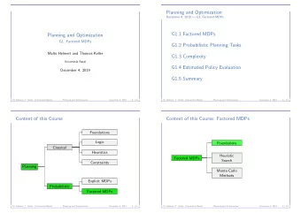
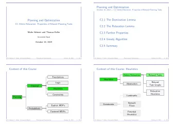
Planning and Optimization

• F2. Bellman Equation & Linear Programming

Malte Helmert and Thomas Keller

Universit¨ at Basel

November 27, 2019

Introduction Bellman Equation Linear Programming Summary

Content of this Course

Planning Classical Foundations Logic Heuristics Constraints Probabilistic Explicit MDPs Factored MDPs

Introduction Bellman Equation Linear Programming Summary

Content of this Course: Explicit MDPs

Explicit MDPs Foundations Linear Programing Policy Iteration Value Iteration

Introduction Bellman Equation Linear Programming Summary

Introduction

Introduction Bellman Equation Linear Programming Summary

Quality of Solutions

Solution in classical planning: plan Optimality criterion of a solution in classical planning: minimize plan cost Solution in probabilistic planning: policy What is the optimality criterion of a solution in probabilistic planning?

Introduction Bellman Equation Linear Programming Summary

Quality of Solutions

Solution in classical planning: plan Optimality criterion of a solution in classical planning: minimize plan cost Solution in probabilistic planning: policy What is the optimality criterion of a solution in probabilistic planning?

Introduction Bellman Equation Linear Programming Summary

Example: Swiss Lotto

Example (Swiss Lotto) What is the expected payoff of placing one bet in Swiss Lotto for a cost of CHF2.50 with (simplified) payouts and probabilities: CHF 30.000.000 with prob. 1/31474716 (6 + 1) CHF 1.000.000 with prob. 1/5245786 (6) CHF 5.000 with prob. 1/850668 (5) CHF 50 with prob. 1/111930 (4) CHF 10 with prob. 1/11480 (3) Solution: 30000000 31474716 + 1000000 5245786 + 5000 850668+ 50 111930 + 10 11480 − 2.5 ≈ −1.35.

Introduction Bellman Equation Linear Programming Summary

Example: Swiss Lotto

Example (Swiss Lotto) What is the expected payoff of placing one bet in Swiss Lotto for a cost of CHF2.50 with (simplified) payouts and probabilities: CHF 30.000.000 with prob. 1/31474716 (6 + 1) CHF 1.000.000 with prob. 1/5245786 (6) CHF 5.000 with prob. 1/850668 (5) CHF 50 with prob. 1/111930 (4) CHF 10 with prob. 1/11480 (3) Solution: 30000000 31474716 + 1000000 5245786 + 5000 850668+ 50 111930 + 10 11480 − 2.5 ≈ −1.35.

Introduction Bellman Equation Linear Programming Summary

Expected Values under Uncertainty

Definition (Expected Value of a Random Variable) Let X be a random variable with a finite number of

• utcomes d1, . . . , dn ∈ R, and let di happen with

probability pi ∈ [0, 1] (for i = 1, . . . n) s.t. n

i=1 pi = 1.

The expected value of X is E[X] = n

i=1(pi · di).

Introduction Bellman Equation Linear Programming Summary

Bellman Equation

Introduction Bellman Equation Linear Programming Summary

Value Functions for MDPs

Definition (Value Functions for MDPs) Let T = S, L, c, T, s0, γ be an MDP and π be an executable policy for T . The state-value Vπ(s) of s under π is defined as Vπ(s) := Qπ(s, π(s)) where the action-value Qπ(s, ℓ) of s and ℓ under π is defined as Qπ(s, ℓ) := R(s, ℓ) + γ ·

• s′∈succ(s,ℓ)

T(s, ℓ, s′) · Vπ(s′). The state-value Vπ(s) describes the expected reward

• f applying π in MDP T , starting from s.

Introduction Bellman Equation Linear Programming Summary

Bellman Equation in MDPs

Definition (Bellman Equation in MDPs) Let T = S, L, c, T, s0, γ be an MDP. The Bellman equation for a state s of T is the set of equations that describes V⋆(s), where V⋆(s) := max

ℓ∈L(s) Q⋆(s, ℓ)

Q⋆(s, ℓ) := R(s, ℓ) + γ ·

• s′∈succ(s,ℓ)

T(s, ℓ, s′) · V⋆(s′). The solution V⋆(s) of the Bellman equation describes the maximal expected reward that can be achieved from state s in MDP T .

Introduction Bellman Equation Linear Programming Summary

Optimal Policy in MDPs

What is the policy that achieves the maximal expected reward? Definition (Optimal Policy in MDPs) Let T = S, L, c, T, s0, γ be an MDP. A policy π is an optimal policy if π(s) ∈ arg maxℓ∈L(s) Q⋆(s, ℓ) for all s ∈ S and the expected reward of π in T is V⋆(s0). W.l.o.g., we assume the optimal policy is unique and written as π⋆.

Introduction Bellman Equation Linear Programming Summary

Value Functions for SSPs

Definition (Value Functions for SSPs) Let T = S, L, c, T, s0, S⋆ be an SSP and π be an executable policy for T . The state-value Vπ(s) of s under π is defined as Vπ(s) :=

• if s ∈ S⋆

Qπ(s, π(s))

• therwise,

where the action-value Qπ(s, ℓ) of s and ℓ under π is defined as Qπ(s, ℓ) := c(ℓ) +

• s′∈succ(s,ℓ)

T(s, ℓ, s′) · Vπ(s′). The state-value Vπ(s) describes the expected cost

• f applying π in SSP T , starting from s.

Introduction Bellman Equation Linear Programming Summary

Bellman Equation in SSPs

Definition (Bellman Equation in SSPs) Let T = S, L, c, T, s0, S⋆ be an SSP. The Bellman equation for a state s of T is the set of equations that describes V⋆(s), where V⋆(s) := min

ℓ∈L(s) Q⋆(s, ℓ)

Q⋆(s, ℓ) := c(ℓ) +

• s′∈succ(s,ℓ)

T(s, ℓ, s′) · V⋆(s′). The solution V⋆(s) of the Bellman equation describes the minimal expected cost that can be achieved from state s in SSP T .

Introduction Bellman Equation Linear Programming Summary

Optimal Policy in SSPs

What is the policy that achieves the minimal expected cost? Definition (Optimal Policy in SSPs) Let T = S, L, c, T, s0, S⋆ be an SSP. A policy π is an optimal policy if π(s) ∈ arg minℓ∈L(s) Q⋆(s, ℓ) for all s ∈ S and the expected cost of π in T is V⋆(s0). W.l.o.g., we assume the optimal policy is unique and written as π⋆.

Introduction Bellman Equation Linear Programming Summary

Proper SSP Policy

Definition (Proper SSP Policy) Let T = S, L, c, T, s0, S⋆ be an SSP and π be an executable policy for T . π is proper if it reaches a goal state from each reachable state with probability 1, i.e. if

• s

p1:ℓ1

− − − →s′,...,s′′ pn:ℓn − − − →s⋆

n

• i=1

pi = 1 for all states s ∈ Sπ(s).

Introduction Bellman Equation Linear Programming Summary

Linear Programming

Introduction Bellman Equation Linear Programming Summary

Content of this Course: Explicit MDPs

Explicit MDPs Foundations Linear Programing Policy Iteration Value Iteration

Introduction Bellman Equation Linear Programming Summary

Linear Programming for SSPs

Bellman equation gives set of equations that describes expected cost for each state there are |S| variables and |S| equations (assuming Q⋆ is replaced in V⋆ with corresponding equation) If we solve these equations, we have solved the SSP Problem: how can we deal with the minimization? ⇒ We have solved the “same” problem before with the help of an LP solver

Introduction Bellman Equation Linear Programming Summary

Reminder: LP for Shortest Path in State Space

Variables Non-negative variable Distances for each state s Objective Maximize Distances0 Subject to Distances⋆= 0 for all goal states s⋆ Distances ≤ Distances′ + c(ℓ) for all transitions s

ℓ

− → s′

Introduction Bellman Equation Linear Programming Summary

LP for Expected Cost in SSP

Variables Non-negative variable ExpCosts for each state s Objective Maximize ExpCosts0 Subject to ExpCosts⋆ = 0 for all goal states s⋆ ExpCosts ≤ (

• s′∈S

T(s, ℓ, s′) · ExpCosts′) + c(ℓ) for all s ∈ S and ℓ ∈ L(s)

Introduction Bellman Equation Linear Programming Summary

LP for Expected Reward in MDP

Variables Non-negative variable ExpRewards for each state s Objective Minimize ExpRewards0 Subject to ExpRewards ≥ (γ ·

• s′∈S

T(s, ℓ, s′)ExpRewards′) + R(s, ℓ) for all s ∈ S and ℓ ∈ L(s)

Introduction Bellman Equation Linear Programming Summary

Complexity of Probabilistic Planning

• ptimal solution for MDPs or SSPs can be

computed with LP solver requires |S| variables and |S| · |L| constraints we know that LPs can be solved in polynomial time ⇒ solving MDPs or SSPs is a polynomial time problem How does this relate to the complexity result for classical planning? Solving MDPs or SSPs is polynomial in |S| · |L|

Introduction Bellman Equation Linear Programming Summary

Complexity of Probabilistic Planning

• ptimal solution for MDPs or SSPs can be

computed with LP solver requires |S| variables and |S| · |L| constraints we know that LPs can be solved in polynomial time ⇒ solving MDPs or SSPs is a polynomial time problem How does this relate to the complexity result for classical planning? Solving MDPs or SSPs is polynomial in |S| · |L|

Introduction Bellman Equation Linear Programming Summary

Summary

Introduction Bellman Equation Linear Programming Summary

Summary

State-value of a policy describes expected reward (cost) of following that policy Related Bellman equation describes optimal policy Solution to Bellman equation gives optimal policy Linear Programming can be used to solve MDPs and SSPs in time polynomial in size of state space and actions