Planning and Optimization G7. Monte-Carlo Tree Search Algorithms - PowerPoint PPT Presentation

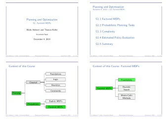
Planning and Optimization G7. Monte-Carlo Tree Search Algorithms (Part I) Malte Helmert and Thomas Keller Universit¨ at Basel December 16, 2019

Introduction Default Policy Optimality MAB Summary Content of this Course Foundations Logic Classical Heuristics Constraints Planning Explicit MDPs Probabilistic Factored MDPs

Introduction Default Policy Optimality MAB Summary Content of this Course: Factored MDPs Foundations Heuristic Factored MDPs Search Suboptimal Algorithms Monte-Carlo Methods MCTS

Introduction Default Policy Optimality MAB Summary Introduction

Introduction Default Policy Optimality MAB Summary Monte-Carlo Tree Search: Reminder Performs iterations with 4 phases: selection: use given tree policy to traverse explicated tree

Introduction Default Policy Optimality MAB Summary Monte-Carlo Tree Search: Reminder Performs iterations with 4 phases: selection: use given tree policy to traverse explicated tree expansion: add node(s) to the tree

Introduction Default Policy Optimality MAB Summary Monte-Carlo Tree Search: Reminder Performs iterations with 4 phases: selection: use given tree policy to traverse explicated tree expansion: add node(s) to the tree simulation: use given default policy to simulate run

Introduction Default Policy Optimality MAB Summary Monte-Carlo Tree Search: Reminder Performs iterations with 4 phases: selection: use given tree policy to traverse explicated tree expansion: add node(s) to the tree simulation: use given default policy to simulate run backpropagation: update visited nodes with Monte-Carlo backups

Introduction Default Policy Optimality MAB Summary Motivation Monte-Carlo Tree Search is a framework of algorithms concrete MCTS algorithms are specified in terms of a tree policy; and a default policy for most tasks, a well-suited MCTS configuration exists but for each task, many MCTS configurations perform poorly and every MCTS configuration that works well in one problem performs poorly in another problem ⇒ There is no “Swiss army knife” configuration for MCTS

Introduction Default Policy Optimality MAB Summary Role of Tree Policy used to traverse explicated tree from root node to a leaf maps decision nodes to a probability distribution over actions (usually as a function over a decision node and its children) exploits information from search tree able to learn over time requires MCTS tree to memorize collected information

Introduction Default Policy Optimality MAB Summary Role of Default Policy used to simulate run from some state to a goal maps states to a probability distribution over actions independent from MCTS tree does not improve over time can be computed quickly constant memory requirements accumulated cost of simulated run used to initialize state-value estimate of decision node

Introduction Default Policy Optimality MAB Summary Default Policy

Introduction Default Policy Optimality MAB Summary MCTS Simulation MCTS simulation with default policy π from state s cost := 0 while s / ∈ S ⋆ : a : ∼ π ( s ) cost := cost + c ( a ) s : ∼ succ( s , a ) return cost Default policy must be proper to guarantee termination of the procedure and a finite cost

Introduction Default Policy Optimality MAB Summary Default Policy: Example Consider deterministic default policy π s State-value of s under π : 60 a 0 : 10 0 . 5 0 5 . u t a 1 : 0 0 . 5 0 . 5 a 2 : 50 v w a 4 : 100 a 3 : 0 g

Introduction Default Policy Optimality MAB Summary Default Policy: Example Consider deterministic default policy π s State-value of s under π : 60 a 0 : 10 Accumulated cost of run: 0 0 . 5 0 5 . u t a 1 : 0 0 . 5 0 . 5 a 2 : 50 v w a 4 : 100 a 3 : 0 g

Introduction Default Policy Optimality MAB Summary Default Policy: Example Consider deterministic default policy π s State-value of s under π : 60 a 0 : 10 Accumulated cost of run: 10 0 . 5 0 5 . u t a 1 : 0 0 . 5 0 . 5 a 2 : 50 v w a 4 : 100 a 3 : 0 g

Introduction Default Policy Optimality MAB Summary Default Policy: Example Consider deterministic default policy π s State-value of s under π : 60 a 0 : 10 Accumulated cost of run: 60 0 . 5 0 5 . u t a 1 : 0 0 . 5 0 . 5 a 2 : 50 v w a 4 : 100 a 3 : 0 g

Introduction Default Policy Optimality MAB Summary Default Policy Realizations Early MCTS implementations used random default policy: � 1 if a ∈ L ( s ) | L ( s ) | π ( a | s ) = 0 otherwise only proper if goal can be reached from each state poor guidance, and due to high variance even misguidance

Introduction Default Policy Optimality MAB Summary Default Policy Realizations There are only few alternatives to random default policy, e.g., heuristic-based policy domain-specific policy Reason: No matter how good the policy, result of simulation can be arbitrarily poor

Introduction Default Policy Optimality MAB Summary Default Policy: Example (2) Consider deterministic default policy π s State-value of s under π : 60 a 0 : 10 Accumulated cost of run: 0 0 . 5 0 5 . u t a 1 : 0 0 . 5 0 . 5 a 2 : 50 v w a 4 : 100 a 3 : 0 g

Introduction Default Policy Optimality MAB Summary Default Policy: Example (2) Consider deterministic default policy π s State-value of s under π : 60 a 0 : 10 Accumulated cost of run: 10 0 . 5 0 5 . u t a 1 : 0 0 . 5 0 . 5 a 2 : 50 v w a 4 : 100 a 3 : 0 g

Introduction Default Policy Optimality MAB Summary Default Policy: Example (2) Consider deterministic default policy π s State-value of s under π : 60 a 0 : 10 Accumulated cost of run: 60 0 . 5 0 5 . u t a 1 : 0 0 . 5 0 . 5 a 2 : 50 v w a 4 : 100 a 3 : 0 g

Introduction Default Policy Optimality MAB Summary Default Policy: Example (2) Consider deterministic default policy π s State-value of s under π : 60 a 0 : 10 Accumulated cost of run: 110 0 . 5 0 5 . u t a 1 : 0 0 . 5 0 . 5 a 2 : 50 v w a 4 : 100 a 3 : 0 g

Introduction Default Policy Optimality MAB Summary Default Policy Realizations Possible solution to overcome this weakness: average over multiple random walks converges to true action-values of policy computationally often very expensive Cheaper and more successful alternative: skip simulation step of MCTS use heuristic directly for initialization of state-value estimates instead of simulating execution of heuristic-guided policy much more successful (e.g. neural networks of AlphaGo)

Introduction Default Policy Optimality MAB Summary Asymptotic Optimality

Introduction Default Policy Optimality MAB Summary Optimal Search Heuristic search algorithms (like AO ∗ or RTDP) are optimal by combining greedy search admissible heuristic Bellman backups In Monte-Carlo Tree Search search behavior defined by tree policy admissibility of default policy / heuristic irrelevant (and usually not given) Monte-Carlo backups MCTS requires different idea for optimal behavior in the limit

Introduction Default Policy Optimality MAB Summary Asymptotic Optimality Asymptotic Optimality Let an MCTS algorithm build an MCTS tree G = � d 0 , D , C , E � . The MCTS algorithm is asymptotically optimal if lim k →∞ ˆ Q k ( c ) = Q ⋆ ( s ( c ) , a ( c )) for all c ∈ C k , where k is the number of trials. this is just one special form of asymptotic optimality some optimal MCTS algorithms are not asymptotically optimal by this definition (e.g., lim k →∞ ˆ Q k ( c ) = ℓ · Q ⋆ ( s ( c ) , a ( c )) for some ℓ ∈ R + ) all practically relevant optimal MCTS algorithms are asymptotically optimal by this definition

Introduction Default Policy Optimality MAB Summary Asymptotically Optimal Tree Policy An MCTS algorithm is asymptotically optimal if 1 its tree policy explores forever: the (infinite) sum of the probabilities that a decision node is visited must diverge ⇒ every search node is explicated eventually and visited infinitely often 2 its tree policy is greedy in the limit: probability that optimal action is selected converges to 1 ⇒ in the limit, backups based on iterations where only an optimal policy is followed dominate suboptimal backups 3 its default policy initializes decision nodes with finite values

Introduction Default Policy Optimality MAB Summary Example: Random Tree Policy Example Consider the random tree policy for decision node d where: � 1 if a ∈ L ( s ( d )) | L ( s ( d )) | π ( a | d ) = 0 otherwise The random tree policy explores forever: Let � d 0 , c 0 , . . . , d n , c n , d � be a sequence of connected nodes in G k and let p := min 0 < i < n − 1 T ( s ( d i ) , a ( c i ) , s ( d i +1 )). Let P k be the probability that d is visited in trial k . With P k ≥ ( 1 | L | · p ) n , we have that k P k ≥ k · ( 1 | L | · p ) n = ∞ � lim k →∞ i =1

Introduction Default Policy Optimality MAB Summary Example: Random Tree Policy Example Consider the random tree policy for decision node d where: � 1 if a ∈ L ( s ( d )) | L ( s ( d )) | π ( a | d ) = 0 otherwise The random tree policy is not greedy in the limit unless all actions are always optimal: The probability that an optimal action a is selected in decision node d is 1 � lim k →∞ 1 − | L ( s ( d )) | < 1 . { a ′ �∈ π V ⋆ ( s ) } � MCTS with random tree policy not asymptotically optimal