Multi-armed Bandits for Efficient Lifetime Estimation in MPSoC - PowerPoint PPT Presentation
Multi-armed Bandits for Efficient Lifetime Estimation in MPSoC Design Calvin Ma, Aditya Mahajan, and Brett H. Meyer Department of Electrical and Computer Engineering McGill University Design Differentiation in DSE Design space exploration
Multi-armed Bandits for Efficient Lifetime Estimation in MPSoC Design Calvin Ma, Aditya Mahajan, and Brett H. Meyer Department of Electrical and Computer Engineering McGill University
Design Differentiation in DSE • Design space exploration (DSE) is often used for MPSoCs • Design spaces are large (on the orders of billions of alternatives) • Design evaluation can be complex (requiring multiple metrics) • Exhaustive search is usually intractable • Goals of DSE: 1. Differentiate poor solutions from good ones 2. Identify the Pareto-optimal set 3. Do so quickly and efficiently 29 March 2017 Brett H. Meyer / McGill University 2
System Lifetime Optimization for MPSoC • Semiconductor scaling has reduced integrated circuit lifetime Electromigration Thermal Cycling Stress migration [Source: JEDEC] • Many strategies have been developed to address failure: • Redundancy (at different granularities) or slack allocation • Thermal management and task migration • System-level optimization seeks to maximize mean time to failure under other constraints (e.g., performance , power , cost ) 29 March 2017 Brett H. Meyer / McGill University 3
Evaluating System Lifetime • Failure mechanisms are modeled mathematically • Historically, with the exponential distribution: easy to work with • Recently, with log-normal and Weibull distributions: more accurate • There is no straightforward closed-form solution for systems of log-normal and Weibull distributions • Therefore, Monte Carlo Simulation (MCS)! • Use failure distributions to generate a random system instance ( sample ) • Determine when that instance fails through simulation • Capture statistics, and repeat! 29 March 2017 Brett H. Meyer / McGill University 4
Multi-armed Bandits for Smarter Estimation • Monte Carlo Simulation is needlessly computationally expensive • Samples are distributed evenly to estimate lifetime • Poor designs are sampled as much as good designs • Multi-armed Bandits (MAB) are smarter • Samples are incrementally distributed in order to differentiate systems • E.g. , to find the best , the best k , etc. • Hypothesis: MAB can achieve DSE goals with fewer evaluations than MCS by differentiating systems, not estimating lifetime 29 March 2017 Brett H. Meyer / McGill University 5
Outline • Multi-armed Bandits • Successive Accept Reject • Gap-based Exploration with Variance • Lifetime Differentiation Experiments and Results • Conclusions and Future Work 29 March 2017 Brett H. Meyer / McGill University 6
Multi-armed Bandits Algorithms • Which slot machine is the best? • Monte Carlo Simulation is systematic • Try every slot machine equally • In the end, compare average payout • Multi-armed Bandits algorithms gamble intelligently [CC BY-SA: Yamaguchi 先生 ] • Try every slot machine, but stay away from bad ones • Do so by managing expected payout from next trial 29 March 2017 Brett H. Meyer / McGill University 7
Simple MAB Example MAB (UCB1) • Assume Bernoulli-distributed MAB(UCB1) on designs with survival probabilities {0.3, 0.5, 0.7, 0.8} systems with different p 1 0.9 • UCB1 plays (samples) the arm 0.8 (system) that maximizes Sample mean 0.7 r 2 ln n 0.6 x i + ¯ 0.5 n i 0.8 • Explore, but favor better arms 0.7 0.4 0.5 0.3 • Eventually, the best system is 0.3 always played 0.2 0 50 100 150 200 250 300 Number of samples (n) 29 March 2017 Brett H. Meyer / McGill University 8
MAB for Lifetime Differentiation • Conventional MAB formulations assume that • The player never stops playing • The reward is incrementally obtained after each arm pull • A single best arm is identified • For DSE, we relax these assumptions • Assume a fixed sample budget used to explore designs • The reward is associated with the final choice • Find the best m arms • Two MAB algorithms can be applied in this context 29 March 2017 Brett H. Meyer / McGill University 9
Successive Accept Reject (SAR) • SAR divides the sample budget into n phases to compare n arms • Each phase, the allocated budget is divided across active arms • After sampling, calculate the distance from boundary between the m good designs and n – m bad ones • Top m designs: ∆ i = ˆ µ i − ˆ µ i ∗ • Bottom n – m designs: ∆ i = ˆ µ i ∗ − ˆ µ i • Remove from consideration the design with the biggest gap 29 March 2017 Brett H. Meyer / McGill University 10
Successive Accept Reject Example • Sample all designs initially Samples per phase for 10 designs, 1000 samples 250 10 Samples per design in current phase • Samples per design grows Number of designs remaining as designs are removed 200 8 • Many samples used to 150 6 differentiate m th and m+1 th designs 100 4 50 2 0 0 1 1 2 2 3 3 4 4 5 5 6 6 7 7 8 8 9 9 10 10 Phase 29 March 2017 Brett H. Meyer / McGill University 11
Successive Accept Reject Example S Successive Accept Rejects (Top 5 out of 10) Successive Accept Rejects (Top 5 out of 10) i A p t R j j t (T ( p 5 t f 10) ) 45 45 40 40 35 35 es le 30 30 pl m am Sa f S 25 25 of e o ge ag 20 20 nt en ce erc 15 15 15 Pe P 10 10 5 5 0 0 0 0 0.1 0 1 0 2 0.2 0 3 0.3 0 4 0.4 0 5 0.5 0 6 0.6 0.7 0 7 0.8 0 8 0 9 0.9 Design Points (ranked from lowest to highest utility) Design Points (ranked from lowest to highest utility) 29 March 2017 Brett H. Meyer / McGill University 12
Gap-based Exploration with Variance (GapE-V) • GapE-V never removes a design from consideration • Instead, pick the design that minimizes the empirical gap with the boundary, plus an exploration factor r 2 a ˆ 7 ab σ i I t = − ∆ i + + 3( T i − 1) T i • Effort is focused near the boundary • High variance, or a limited number of samples, increase likelihood a design is sampled 29 March 2017 Brett H. Meyer / McGill University 13
GapE-V Example G GapE (Top 5 out of 10) GapE (Top 5 out of 10) p ( E (T p 5 t f 10) ) 25 25 20 20 es le pl m am 15 15 Sa f S of e o ge ag nt 10 10 en ce erc Pe P 5 0 0 0 0 0 1 0.1 0.2 0 2 0 3 0.3 0.4 0 4 0.5 0 5 0 6 0.6 0 7 0.7 0 8 0.8 0 9 0.9 Design Points (ranked from lowest to highest utility) Design Points (ranked from lowest to highest utility) 29 March 2017 Brett H. Meyer / McGill University 14
Experimental Setup • NoC-based MPSoC lifetime optimization with slack allocation • Slack is spare compute and storage capacity • Add slack to components s.t. remapping mitigates one or more failures • Two applications, two architectures each ARM9 ARM11 64KB M3 M3 BSP- Drng VCV2 Rcns Pad2 VLD • Component library of processors, SRAMs 1 2 3 4 256KB 64KB M3 M3 96KB VMV VBV/ ARM11 Pad1 Dblk VCV3 VCV1 S/M/T MPEG-4: 140K designs ARM9 M3 1MB 1MB M3 1MB 1MB ARM9 Processor Jug2 In Mem1 Mem2 In Mem1 Mem2 Jug2 1 1 2 ARM9 ARM11 64KB 64KB BSP- M3 S/M/T M3 VBV/ VCV2 ARM11 ARM11 VLD HVS HVS VCV1 M3 1MB M3 1MB Memory NR NR 1 2 HS Mem3 HS Mem3 Switch 2 3 4 3 256KB M3 M3 M3 M3 M3 VMV M3 M3 M3 ARM11 ARM11 Dblk Rcns VS SE Blend VS SE Blend Jug1 Jug1 5 4 3 MWD: 11K designs M3 M3 96KB ARM11 Pad1 Pad2 VCV3 29 March 2017 Brett H. Meyer / McGill University Drng 15
Evaluating the Chosen m • We compare SAR, GapE-V, and MCS • Optimal set determined with MCS using 1M samples per design • How likely is it that an approach picks the wrong set? • Compare the aggregate MTTF using policy J and the optimal set m � X µ ∗ Pr i − E µ J ( i ) > ✏ ≤ � i =1 is the probability of identification error , the chance a subset of • δ m differs significantly from the optimal set 29 March 2017 Brett H. Meyer / McGill University 16
Picking the Top 50, MWD MWD3S, m=50 MWD4S, m=50 0 0 10 10 Confidence parameter δ Confidence parameter δ MCS MCS SAR SAR GAPE GAPE − 1 − 1 10 10 − 2 − 2 10 10 100 200 300 400 500 100 200 300 400 500 Samples Samples 29 March 2017 Brett H. Meyer / McGill University 17
Picking the Top 50, MPEG-4 MPEG4S, m=50 MPEG5S, m=50 0 0 10 10 Confidence parameter δ Confidence parameter δ MCS MCS SAR SAR GAPE GAPE − 1 − 1 10 10 − 2 − 2 10 10 100 200 300 400 500 100 200 300 400 500 Samples Samples 29 March 2017 Brett H. Meyer / McGill University 18
Comparison with MCS after 500 samples m=20 m=30 Benchmark δ SAR GapE-V δ SAR GapE-V MWD3S 0.002 1.92x 1.72x 0.003 1.72x 1.71x MWD4S 0.071 3.33x 2.13x 0.112 2.96x 2.07x MPEG4S 0.120 3.57x 2.70x 0.101 3.52x 2.48x MPEG5S 0.052 5.26x 3.57x 0.083 4.07x 3.05x m=40 m=50 Benchmark δ SAR GapE-V δ SAR GapE-V MWD3S 0.009 1.79x 1.67x 0.021 1.49x 1.45x MWD4S 0.180 2.54x 2.01x 0.148 2.44x 1.92x MPEG4S 0.202 3.60x 2.43x 0.115 3.33x 2.27x MPEG5S 0.292 3.70x 3.07x 0.162 3.57x 2.86x 29 March 2017 Brett H. Meyer / McGill University 19
Recommend
More recommend
Explore More Topics
Stay informed with curated content and fresh updates.
