Plan of the Lecture Review: rules for sketching root loci; - PowerPoint PPT Presentation
Plan of the Lecture Review: rules for sketching root loci; introduction to dynamic compensation Todays topic: lead and lag dynamic compensation Plan of the Lecture Review: rules for sketching root loci; introduction to dynamic
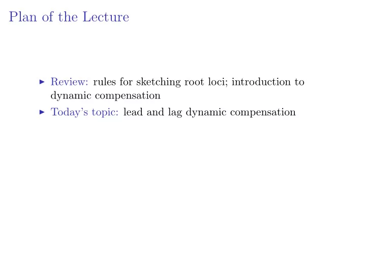
Plan of the Lecture ◮ Review: rules for sketching root loci; introduction to dynamic compensation ◮ Today’s topic: lead and lag dynamic compensation
Plan of the Lecture ◮ Review: rules for sketching root loci; introduction to dynamic compensation ◮ Today’s topic: lead and lag dynamic compensation Goal: introduce the use of lead and lag dynamic compensators for approximate implementation of PD and PI control.
Plan of the Lecture ◮ Review: rules for sketching root loci; introduction to dynamic compensation ◮ Today’s topic: lead and lag dynamic compensation Goal: introduce the use of lead and lag dynamic compensators for approximate implementation of PD and PI control. Reading: FPE, Chapter 5
From Last Time: Double Integrator with PD-Control 1 + K · s + 1 Characteristic equation: = 0 s 2 1.0 0.5 - 3.5 - 3.0 - 2.5 - 2.0 - 1.5 - 1.0 - 0.5 - 0.5 - 1.0
From Last Time: Double Integrator with PD-Control 1 + K · s + 1 Characteristic equation: = 0 s 2 1.0 0.5 - 3.5 - 3.0 - 2.5 - 2.0 - 1.5 - 1.0 - 0.5 - 0.5 - 1.0 What can we conclude from this root locus about stabilization?
From Last Time: Double Integrator with PD-Control 1 + K · s + 1 Characteristic equation: = 0 s 2 1.0 0.5 - 3.5 - 3.0 - 2.5 - 2.0 - 1.5 - 1.0 - 0.5 - 0.5 - 1.0 What can we conclude from this root locus about stabilization? ◮ all closed-loop poles are in LHP (we already knew this from Routh, but now can visualize)
From Last Time: Double Integrator with PD-Control 1 + K · s + 1 Characteristic equation: = 0 s 2 1.0 0.5 - 3.5 - 3.0 - 2.5 - 2.0 - 1.5 - 1.0 - 0.5 - 0.5 - 1.0 What can we conclude from this root locus about stabilization? ◮ all closed-loop poles are in LHP (we already knew this from Routh, but now can visualize) ◮ nice damping, so can meet reasonable specs
From Last Time: Double Integrator with PD-Control 1 + K · s + 1 Characteristic equation: = 0 s 2 1.0 0.5 - 3.5 - 3.0 - 2.5 - 2.0 - 1.5 - 1.0 - 0.5 - 0.5 - 1.0 What can we conclude from this root locus about stabilization? ◮ all closed-loop poles are in LHP (we already knew this from Routh, but now can visualize) ◮ nice damping, so can meet reasonable specs So, the effect of D-gain was to introduce an open-loop zero into LHP, and this zero “pulled” the root locus into LHP, thus stabilizing the system.
Dynamic Compensation Objectives: stabilize the system and satisfy given time response specs using a stable, causal controller. K s + z 1 + R Y s + p s 2 − Characteristic equation: 1 + K · s + z s + p · 1 s 2 = 1 + KL ( s ) = 0
Approximate PD Using Dynamic Compensation Reminder: we can approximate the D-controller K D s by ps K D → K D s as p → ∞ s + p − — here, − p is the pole of the controller.
Approximate PD Using Dynamic Compensation Reminder: we can approximate the D-controller K D s by ps K D → K D s as p → ∞ s + p − — here, − p is the pole of the controller. So, we replace the PD controller K P + K D s by ps K ( s ) = K P + K D s + p
Approximate PD Using Dynamic Compensation Reminder: we can approximate the D-controller K D s by ps K D → K D s as p → ∞ s + p − — here, − p is the pole of the controller. So, we replace the PD controller K P + K D s by ps K ( s ) = K P + K D s + p + E U R K ( s ) G ( s ) Y − controller plant
Approximate PD Using Dynamic Compensation Reminder: we can approximate the D-controller K D s by ps K D → K D s as p → ∞ s + p − — here, − p is the pole of the controller. So, we replace the PD controller K P + K D s by ps K ( s ) = K P + K D s + p + E U R K ( s ) G ( s ) Y − controller plant � � ps Closed-loop poles: 1 + K P + K D G ( s ) = 0 s + p
Lead & Lag Compensators Consider a general controller of the form K s + z — K, z, p > 0 are design parameters s + p
Lead & Lag Compensators Consider a general controller of the form K s + z — K, z, p > 0 are design parameters s + p Depending on the relative values of z and p , we call it:
Lead & Lag Compensators Consider a general controller of the form K s + z — K, z, p > 0 are design parameters s + p Depending on the relative values of z and p , we call it: ◮ a lead compensator when z < p
Lead & Lag Compensators Consider a general controller of the form K s + z — K, z, p > 0 are design parameters s + p Depending on the relative values of z and p , we call it: ◮ a lead compensator when z < p ◮ a lag compensator when z > p
Lead & Lag Compensators Consider a general controller of the form K s + z — K, z, p > 0 are design parameters s + p Depending on the relative values of z and p , we call it: ◮ a lead compensator when z < p ◮ a lag compensator when z > p Why the name “lead/lag?” — think frequency response
Lead & Lag Compensators Consider a general controller of the form K s + z — K, z, p > 0 are design parameters s + p Depending on the relative values of z and p , we call it: ◮ a lead compensator when z < p ◮ a lag compensator when z > p Why the name “lead/lag?” — think frequency response ∠ jω + z jω + p = ∠ ( jω + z ) − ∠ ( jω + p ) = ψ − φ
Lead & Lag Compensators Consider a general controller of the form K s + z — K, z, p > 0 are design parameters s + p Depending on the relative values of z and p , we call it: ◮ a lead compensator when z < p ◮ a lag compensator when z > p Why the name “lead/lag?” — think frequency response ∠ jω + z jω + p = ∠ ( jω + z ) − ∠ ( jω + p ) = ψ − φ ◮ if z < p , then ψ − φ > 0 (phase lead) ω ◮ if z > p , then ψ − φ < 0 ψ φ (phase lag) z p
Back to Double Integrator K s + z 1 + Y R s + p s 2 − Controller transfer function is K s + z s + p , where: pK P K = K P + pK D , z = K P + pK D
Back to Double Integrator K s + z 1 + Y R s + p s 2 − Controller transfer function is K s + z s + p , where: pK P → K P p →∞ K = K P + pK D , z = − − − K P + pK D K D
Back to Double Integrator K s + z 1 + Y R s + p s 2 − Controller transfer function is K s + z s + p , where: pK P → K P p →∞ K = K P + pK D , z = − − − K P + pK D K D so, as p → ∞ , z tends to a constant, so we get a lead controller.
Back to Double Integrator K s + z 1 + Y R s + p s 2 − Controller transfer function is K s + z s + p , where: pK P → K P p →∞ K = K P + pK D , z = − − − K P + pK D K D so, as p → ∞ , z tends to a constant, so we get a lead controller. We use lead controllers as dynamic compensators for approximate PD control.
Double Integrator & Lead Compensator K s + z 1 + Y R s + p s 2 −
Double Integrator & Lead Compensator K s + z 1 + Y R s + p s 2 − To keep things simple, let’s set K P = K D . Then:
Double Integrator & Lead Compensator K s + z 1 + Y R s + p s 2 − To keep things simple, let’s set K P = K D . Then: K = K P + pK D = (1 + p ) K D
Double Integrator & Lead Compensator K s + z 1 + Y R s + p s 2 − To keep things simple, let’s set K P = K D . Then: K = K P + pK D = (1 + p ) K D pK P z = K P + pK D
Double Integrator & Lead Compensator K s + z 1 + Y R s + p s 2 − To keep things simple, let’s set K P = K D . Then: K = K P + pK D = (1 + p ) K D pK P pK D z = = K P + pK D (1 + p ) K D
Double Integrator & Lead Compensator K s + z 1 + Y R s + p s 2 − To keep things simple, let’s set K P = K D . Then: K = K P + pK D = (1 + p ) K D pK P pK D p z = = = K P + pK D (1 + p ) K D 1 + p
Double Integrator & Lead Compensator K s + z 1 + Y R s + p s 2 − To keep things simple, let’s set K P = K D . Then: K = K P + pK D = (1 + p ) K D pK P pK D p p →∞ z = = = → 1 − − − K P + pK D (1 + p ) K D 1 + p Since we can choose p and z directly, let’s take z = 1 and p large .
Double Integrator & Lead Compensator K s + z 1 + Y R s + p s 2 − To keep things simple, let’s set K P = K D . Then: K = K P + pK D = (1 + p ) K D pK P pK D p p →∞ z = = = → 1 − − − K P + pK D (1 + p ) K D 1 + p Since we can choose p and z directly, let’s take z = 1 and p large . We expect to get behavior similar to PD control.
Double Integrator & Lead Compensator + K L ( s ) R Y − L ( s ) = s + z s + p · 1 s + 1 z =1 = s 2 s 2 ( s + p )
Double Integrator & Lead Compensator + K L ( s ) R Y − L ( s ) = s + z s + p · 1 s + 1 z =1 = s 2 s 2 ( s + p ) Let’s try a few values of p . Here’s p = 10:
Double Integrator & Lead Compensator + K L ( s ) R Y − L ( s ) = s + z s + p · 1 s + 1 z =1 = s 2 s 2 ( s + p ) Let’s try a few values of p . Here’s p = 10: 2 1 - 10 - 8 - 6 - 4 - 2 - 1 - 2
Double Integrator & Lead Compensator + K L ( s ) R Y − L ( s ) = s + z s + p · 1 s + 1 z =1 = s 2 s 2 ( s + p ) Let’s try a few values of p . Here’s p = 10: 2 1 - 10 - 8 - 6 - 4 - 2 - 1 - 2 Close to j ω -axis, this root locus looks similar to the PD root locus. However, the pole at s = − 10 makes the locus look different for s far into LHP.
Double Integrator & Lead Compensator s + 1 L ( s ) = s 2 ( s + p ) Root locus for p = 10: 2 1 - 10 - 8 - 6 - 4 - 2 - 1 - 2
Recommend
More recommend
Explore More Topics
Stay informed with curated content and fresh updates.
