Particle Monte Carlo methods in statistical learning and rare event - PowerPoint PPT Presentation

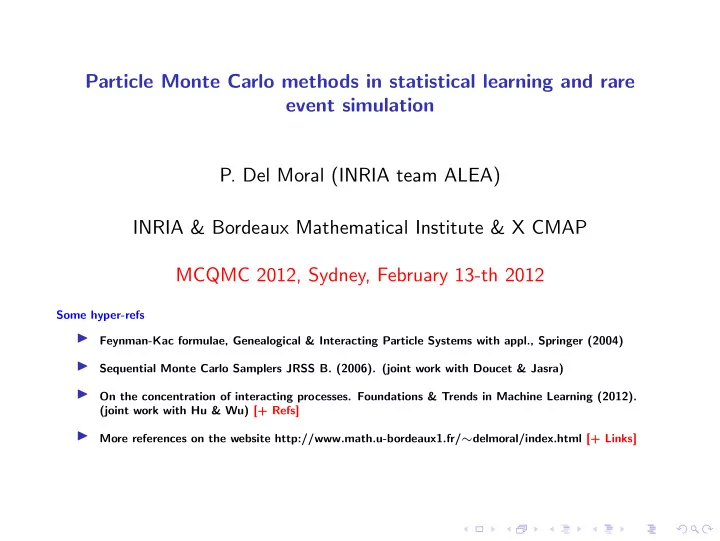
Particle Monte Carlo methods in statistical learning and rare event simulation P. Del Moral (INRIA team ALEA) INRIA & Bordeaux Mathematical Institute & X CMAP MCQMC 2012, Sydney, February 13-th 2012 Some hyper-refs ◮ Feynman-Kac formulae, Genealogical & Interacting Particle Systems with appl., Springer (2004) ◮ Sequential Monte Carlo Samplers JRSS B. (2006). (joint work with Doucet & Jasra) ◮ On the concentration of interacting processes. Foundations & Trends in Machine Learning (2012). (joint work with Hu & Wu) [+ Refs] ◮ More references on the website http://www.math.u-bordeaux1.fr/ ∼ delmoral/index.html [+ Links]

Stochastic particle sampling methods Interacting jumps models Genetic type interacting particle models Particle Feynman-Kac models The 4 particle estimates Island particle models ( ⊂ Parallel Computing) Bayesian statistical learning Nonlinear filtering models Fixed parameter estimation in HMM models Particle stochastic gradient models Approximate Bayesian Computation Interacting Kalman-Filters Uncertainty propagations in numerical codes Concentration inequalities Current population models Particle free energy Genealogical tree models Backward particle models

Stochastic particle sampling methods Interacting jumps models Genetic type interacting particle models Particle Feynman-Kac models The 4 particle estimates Island particle models ( ⊂ Parallel Computing) Bayesian statistical learning Concentration inequalities

Introduction Stochastic particle methods = Universal adaptive sampling technique 2 types of stochastic interacting particle models: ◮ Diffusive particle models with mean field drifts [McKean-Vlasov style] ◮ Interacting jump particle models [Boltzmann & Feynman-Kac style]

Lectures ⊂ Interacting jumps models ◮ Interacting jumps = Recycling transitions = ◮ Discrete time models ( ⇔ geometric rejection/jump times)

Genetic type interacting particle models ◮ Mutation-Proposals w.r.t. Markov transitions X n − 1 � X n ∈ E n . ◮ Selection-Rejection-Recycling w.r.t. potential/fitness function G n .

Equivalent particle algorithms Sequential Monte Carlo Sampling Resampling Particle Filters Prediction Updating Genetic Algorithms Mutation Selection Evolutionary Population Exploration Branching-selection Diffusion Monte Carlo Free evolutions Absorption Quantum Monte Carlo Walkers motions Reconfiguration Sampling Algorithms Transition proposals Accept-reject-recycle

Equivalent particle algorithms Sequential Monte Carlo Sampling Resampling Particle Filters Prediction Updating Genetic Algorithms Mutation Selection Evolutionary Population Exploration Branching-selection Diffusion Monte Carlo Free evolutions Absorption Quantum Monte Carlo Walkers motions Reconfiguration Sampling Algorithms Transition proposals Accept-reject-recycle More botanical names: bootstrapping, spawning, cloning, pruning, replenish, multi-level splitting, enrichment, go with the winner, . . . 1950 ≤ Meta-Heuristic style stochastic algorithms ≤ 1996

A single stochastic model Particle interpretation of Feynman-Kac path integrals

Genealogical tree evolution (Population size, Time horizon)=( N , n ) = (3 , 3) ✲ • ✲ • = • • • ✲ ✲ • • • • = • ✲ ✲ ✲ ✲ • • • • = • ✲

Genealogical tree evolution (Population size, Time horizon)=( N , n ) = (3 , 3) ✲ • ✲ • = • • • ✲ ✲ • • • • = • ✲ ✲ ✲ ✲ • • • • = • ✲ Meta-heuristics � ”Meta-Theorem” : Ancestral lines ≃ i.i.d. samples w.r.t. Feynman-Kac measure   Q n := 1   � G p ( X p ) P n with P n := Law ( X 0 , . . . , X n ) Z n   0 ≤ p < n

Genealogical tree evolution (Population size, Time horizon)=( N , n ) = (3 , 3) ✲ • ✲ • = • • • ✲ ✲ • • • • = • ✲ ✲ ✲ ✲ • • • • = • ✲ Meta-heuristics � ”Meta-Theorem” : Ancestral lines ≃ i.i.d. samples w.r.t. Feynman-Kac measure   Q n := 1   � G p ( X p ) P n with P n := Law ( X 0 , . . . , X n ) Z n   0 ≤ p < n Example G n = 1 A n → Q n = Law (( X 0 , . . . , X n ) | X p ∈ A p , p < n )

Particle estimates More formally � � ξ i 0 , n , ξ i 1 , n , . . . , ξ i := i -th ancetral line of the i -th current individual = ξ i n , n n ⇓ 1 � n , n ) − → N →∞ Q n δ ( ξ i 0 , n ,ξ i 1 , n ,...,ξ i N 1 ≤ i ≤ N

Particle estimates More formally � � ξ i 0 , n , ξ i 1 , n , . . . , ξ i := i -th ancetral line of the i -th current individual = ξ i n , n n ⇓ 1 � n , n ) − → N →∞ Q n δ ( ξ i 0 , n ,ξ i 1 , n ,...,ξ i N 1 ≤ i ≤ N ⊕ Current population models n := 1 � η N n − → N →∞ η n = n -th time marginal of Q n δ ξ i N 1 ≤ i ≤ N

Particle estimates More formally � � ξ i 0 , n , ξ i 1 , n , . . . , ξ i := i -th ancetral line of the i -th current individual = ξ i n , n n ⇓ 1 � n , n ) − → N →∞ Q n δ ( ξ i 0 , n ,ξ i 1 , n ,...,ξ i N 1 ≤ i ≤ N ⊕ Current population models n := 1 � η N n − → N →∞ η n = n -th time marginal of Q n δ ξ i N 1 ≤ i ≤ N ⊕ Unbiased particle approximation   �  � � Z N η N  = n = p ( G p ) − → N →∞ Z n = E G p ( X p ) η p ( G p ) 0 ≤ p < n 0 ≤ p < n 0 ≤ p < n

Particle estimates More formally � � ξ i 0 , n , ξ i 1 , n , . . . , ξ i := i -th ancetral line of the i -th current individual = ξ i n , n n ⇓ 1 � n , n ) − → N →∞ Q n δ ( ξ i 0 , n ,ξ i 1 , n ,...,ξ i N 1 ≤ i ≤ N ⊕ Current population models n := 1 � η N n − → N →∞ η n = n -th time marginal of Q n δ ξ i N 1 ≤ i ≤ N ⊕ Unbiased particle approximation   �  � � Z N η N  = n = p ( G p ) − → N →∞ Z n = E G p ( X p ) η p ( G p ) 0 ≤ p < n 0 ≤ p < n 0 ≤ p < n n = � proportion of success − Ex.: G n = 1 A n � Z N → P ( X p ∈ A p , p < n )

� n := 1 Illustration : η n ≃ η N 1 ≤ i ≤ N δ ξ i N n

� n := 1 Illustration : η n ≃ η N 1 ≤ i ≤ N δ ξ i N n

� n := 1 Illustration : η n ≃ η N 1 ≤ i ≤ N δ ξ i N n

� n := 1 Illustration : η n ≃ η N 1 ≤ i ≤ N δ ξ i N n

� n := 1 Illustration : η n ≃ η N 1 ≤ i ≤ N δ ξ i N n

� n := 1 Illustration : η n ≃ η N 1 ≤ i ≤ N δ ξ i N n

� n := 1 Illustration : η n ≃ η N 1 ≤ i ≤ N δ ξ i N n

� n := 1 Illustration : η n ≃ η N 1 ≤ i ≤ N δ ξ i N n

� n := 1 Illustration : η n ≃ η N 1 ≤ i ≤ N δ ξ i N n

� n := 1 Illustration : η n ≃ η N 1 ≤ i ≤ N δ ξ i N n

� n := 1 Illustration : η n ≃ η N 1 ≤ i ≤ N δ ξ i N n

� n := 1 Illustration : η n ≃ η N 1 ≤ i ≤ N δ ξ i N n

� n := 1 Illustration : η n ≃ η N 1 ≤ i ≤ N δ ξ i N n

� n := 1 Illustration : η n ≃ η N 1 ≤ i ≤ N δ ξ i N n

� n := 1 Illustration : η n ≃ η N 1 ≤ i ≤ N δ ξ i N n

� n := 1 Illustration : η n ≃ η N 1 ≤ i ≤ N δ ξ i N n

� n := 1 Illustration : η n ≃ η N 1 ≤ i ≤ N δ ξ i N n

� n := 1 Illustration : η n ≃ η N 1 ≤ i ≤ N δ ξ i N n

� n := 1 Illustration : η n ≃ η N 1 ≤ i ≤ N δ ξ i N n

Complete ancestral tree when M n ( x , dy ) = H n ( x , y ) λ ( dy ) Backward Markov chain model Q N n ( d ( x 0 , . . . , x n )) := η N n ( dx n ) M n ,η N n − 1 ( x n , dx n − 1 ) . . . M 1 ,η N 0 ( x 1 , dx 0 ) with the random particle matrices: n ( x n +1 , dx n ) ∝ η N M n +1 ,η N n ( dx n ) G n ( x n ) H n +1 ( x n , x n +1 )

Complete ancestral tree when M n ( x , dy ) = H n ( x , y ) λ ( dy ) Backward Markov chain model Q N n ( d ( x 0 , . . . , x n )) := η N n ( dx n ) M n ,η N n − 1 ( x n , dx n − 1 ) . . . M 1 ,η N 0 ( x 1 , dx 0 ) with the random particle matrices: n ( x n +1 , dx n ) ∝ η N M n +1 ,η N n ( dx n ) G n ( x n ) H n +1 ( x n , x n +1 ) Example: Normalized additive functionals 1 � f n ( x 0 , . . . , x n ) = f p ( x p ) n + 1 0 ≤ p ≤ n ⇓ 1 � Q N η N n ( f n ) := n M n ,η N n − 1 . . . M p +1 ,η N p ( f p ) n + 1 0 ≤ p ≤ n � �� � matrix operations

Island models ( ⊂ Parallel Computing) Reminder : the unbiased property     � �  η N η N E  f n ( X n ) G p ( X p ) = E n ( f n ) p ( G p )   0 ≤ p < n 0 ≤ p < n   � =  F n ( X n ) G p ( X p ) E  0 ≤ p < n with the Island evolution Markov chain model X n := η N G n ( X n ) = η N n ( G n ) = X n ( G n ) and n ⇓ particle model with ( X n , G n ( X n )) = Interacting Island particle model

Stochastic particle sampling methods Bayesian statistical learning Nonlinear filtering models Fixed parameter estimation in HMM models Particle stochastic gradient models Approximate Bayesian Computation Interacting Kalman-Filters Uncertainty propagations in numerical codes Concentration inequalities

Bayesian statistical learning