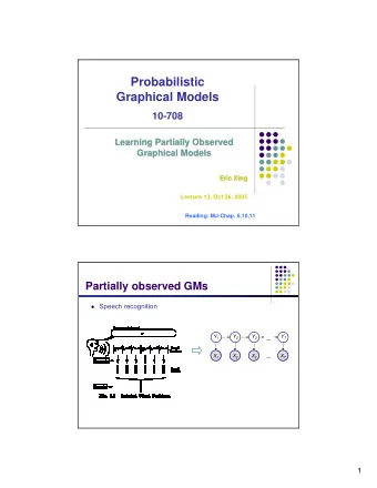
Partially observed GMs Speech recognition Y 1 Y 2 Y 3 Y T ... X 1 - PDF document

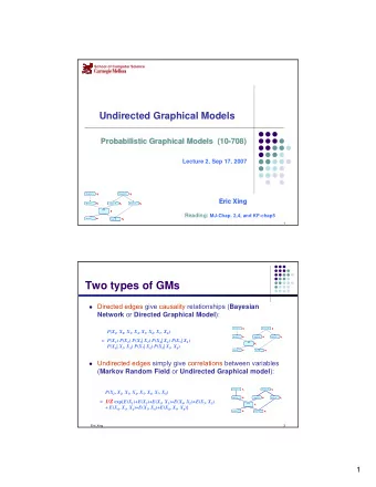
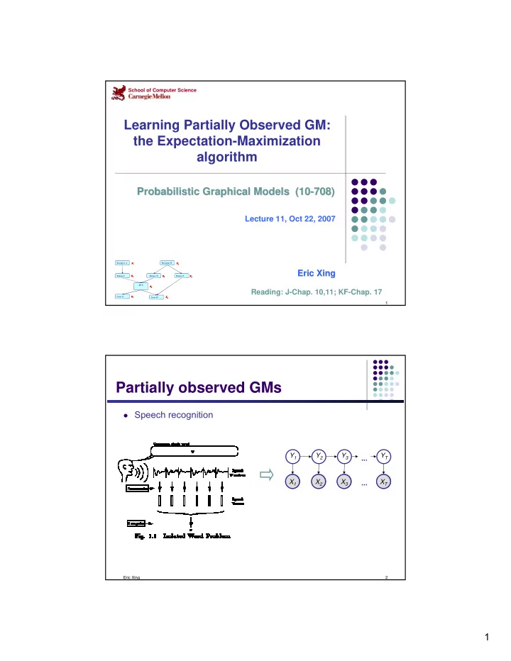
School of Computer Science Learning Partially Observed GM: the Expectation-Maximization algorithm Probabilistic Graphical Models (10- Probabilistic Graphical Models (10 -708) 708) Lecture 11, Oct 22, 2007 Receptor A Receptor A Receptor B Receptor B X 1 X 1 X 1 X 2 X 2 X 2 Eric Xing Eric Xing Kinase C Kinase C X 3 X 3 X 3 Kinase D Kinase D X 4 X 4 X 4 Kinase E Kinase E X 5 X 5 X 5 TF F TF F X 6 X 6 X 6 Reading: J-Chap. 10,11; KF-Chap. 17 Gene G Gene G X 7 X 7 X 7 Gene H Gene H X 8 X 8 X 8 1 Partially observed GMs � Speech recognition Y 1 Y 2 Y 3 Y T ... X 1 A X 2 A X 3 A ... X T A Eric Xing 2 1

Partially observed GM � Biological Evolution ancestor ? T years Q m Q h G A A G C A C A Eric Xing 3 Mixture models � A density model p ( x ) may be multi-modal. � We may be able to model it as a mixture of uni-modal distributions (e.g., Gaussians). � Each mode may correspond to a different sub-population (e.g., male and female). Eric Xing 4 2

Unobserved Variables � A variable can be unobserved (latent) because: it is an imaginary quantity meant to provide some simplified and � abstractive view of the data generation process e.g., speech recognition models, mixture models … � it is a real-world object and/or phenomena, but difficult or impossible to � measure e.g., the temperature of a star, causes of a disease, evolutionary � ancestors … it is a real-world object and/or phenomena, but sometimes wasn’t � measured, because of faulty sensors, etc. � Discrete latent variables can be used to partition/cluster data into sub-groups. � Continuous latent variables (factors) can be used for dimensionality reduction (factor analysis, etc). Eric Xing 5 Gaussian Mixture Models (GMMs) � Consider a mixture of K Gaussian components: ∑ µ Σ = π µ Σ ( , ) ( , | , ) p x N x n k k k k mixture proportion mixture component � This model can be used for unsupervised clustering. This model (fit by AutoClass) has been used to discover new kinds of � stars in astronomical data, etc. Eric Xing 6 3

Gaussian Mixture Models (GMMs) � Consider a mixture of K Gaussian components: Z Z is a latent class indicator vector: � ( ) ∏ k = π = π z X p ( z ) multi ( z : ) n n n k k X is a conditional Gaussian variable with a class-specific mean/covariance � 1 { } 1 − 1 = µ Σ = 1 µ Σ µ k T p ( x | z , , ) exp - ( x - ) ( x - ) 2 1 2 n n 2 2 n k k n k π Σ / m / ( ) k The likelihood of a sample: � mixture component mixture proportion ∑ 1 1 µ Σ = = π = µ Σ k k p ( x , ) p ( z | ) p ( x , | z , , ) n ( ) ∑ k ∑ ∏ ( ) k = π µ Σ k = π µ Σ z z ( : , ) ( , | , ) n N x n N x k n k k k k k z k k n Eric Xing 7 Why is Learning Harder? � In fully observed iid settings, the log likelihood decomposes into a sum of local terms (at least for directed models). θ = θ = θ + θ l ( ; ) log ( , | ) log ( | ) log ( | , ) D p x z p z p x z c z x � With latent variables, all the parameters become coupled together via marginalization ∑ ∑ l θ = θ = θ θ ( ; ) log ( , | ) log ( | ) ( | , ) D p x z p z p x z c z x z z Eric Xing 8 4

Toward the EM algorithm � Recall MLE for completely observed data z i � Data log-likelihood x i ∏ N ∏ = = π µ σ l θ ( ; ) log ( , ) log ( | ) ( | , , ) D p z x p z p x z n n n n n n n ∑ ∑ ∏ ∏ = π k + µ σ k z z log log ( ; , ) n N x n k n k n k n k ∑∑ ∑∑ 2 = π 1 µ + k k z log - z ( x - ) C 2 2 n k n σ n k n k n k � MLE π = l θ ˆ , arg max ( ; D ), π ∑ k MLE k z x µ = l ⇒ µ = n n θ ˆ , arg max ( ; ) ˆ n D ∑ µ k MLE k , MLE k z n σ = l n θ ˆ , arg max ( ; ) D σ k MLE � What if we do not know z n ? Eric Xing 9 Recall: K-means − 1 = − µ Σ − µ ( t ) ( t ) T ( t ) ( t ) z arg max ( x ) ( x ) n n k k n k k ∑ δ ( ) t ( , ) z k x 1 µ + = n n ( ) t n ∑ δ k ( t ) ( , ) z k n n Eric Xing 10 5

Expectation-Maximization � Start: "Guess" the centroid µ k and coveriance Σ k of each of the K clusters � � Loop Eric Xing 11 Example: Gaussian mixture model A mixture of K Gaussians: � Z n Z is a latent class indicator vector � ( ) k ∏ z p z = z π = π X n n ( ) multi ( : ) n n k k N X is a conditional Gaussian variable with class-specific mean/covariance � 1 { } p x z 1 x x k = µ Σ = 1 µ T Σ − 1 µ ( | , , ) exp - ( - ) ( - ) n n 2 n k k n k 1 2 2 π m 2 Σ / / ( ) k The likelihood of a sample: � ∑ p x µ Σ = p z k = 1 π p x z k = 1 µ Σ ( , ) ( | ) ( , | , , ) n k ( ) ∑ ∑ ∏ ( ) k z N x z k N x = π µ Σ = π µ Σ n ( : , ) n ( , | , ) k n k k k k k z k k n The expected complete log likelihood � ∑ ∑ x z p z p x z = π + µ Σ l θ ( ; , ) log ( | ) log ( | , , ) c n n n p z x p z x ( | ) ( | ) n n ( ) ∑∑ ∑∑ 1 z k z k x T − 1 x C = π − − µ Σ − µ + Σ + log ( ) ( ) log n k n n k k n k k 2 n k n k Eric Xing 12 6

E-step l ( θ � We maximize iteratively using the following ) c iterative procedure: ─ Expectation step: computing the expected value of the sufficient statistics of the hidden variables (i.e., z ) given current est. of the parameters (i.e., π and µ ). t N x t t π µ Σ ( ) ( ) ( ) ( , | , ) k t z k p z k 1 x t t τ = = = µ Σ = k n k k ( ) ( ) ( ) ( | , , ) ∑ n n n t t N x t t q π µ Σ ( ) ( ) ( ) ( ) ( , | , ) i n i i i � Here we are essentially doing inference Eric Xing 13 M-step l � We maximize iteratively using the following ( θ ) c iterative procudure: ─ Maximization step: compute the parameters under current results of the expected value of the hidden variables ∑ ⇒ 0 ∀ 1 π = ∂ = π = * θ θ arg max ( ) , ( ) , , s.t. l l k ∂ π k c c k k k ∑ ∑ τ k z ( ) k t n ⇒ n π = ( ) = = * n t n q k n N N N k ∑ τ k ( t ) x ⇒ + 1 µ = µ = n n * θ ( t ) n arg max l ( ) , ∑ Fact : k k τ k ( t ) 1 ∂ − n log A n = T ∑ A 1 1 ∂ − 1 τ − µ + − µ + k ( t ) ( t ) ( t ) T A ( x )( x ) ⇒ 1 Σ = Σ + = n n k n k * θ ( t ) n T arg max l ( ) , ∑ ∂ x x A T k k τ = k ( t ) xx ∂ n A n This is isomorphic to MLE except that the variables that are hidden are � replaced by their expectations (in general they will by replaced by their corresponding " sufficient statistics ") Eric Xing 14 7

Compare: K-means and EM The EM algorithm for mixtures of Gaussians is like a "soft version" of the K-means algorithm. K-means EM � � In the K-means “E-step” we do hard E-step � � assignment: τ = k ( t ) k z n n ( ) t − 1 q = − µ Σ − µ ( t ) ( t ) T ( t ) ( t ) z arg max ( x ) ( x ) n n k k n k π µ Σ ( t ) ( t ) ( t ) N ( x , | , ) k 1 = = µ Σ = k ( t ) ( t ) p ( z | x , , ) ∑ k n k k n π µ Σ ( t ) ( t ) ( t ) ( , | , ) N x i n i i In the K-means “M-step” we update the � i means as the weighted sum of the data, but now the weights are 0 or 1: M-step � ∑ ∑ τ δ k ( t ) ( t ) x ( z , k ) x + 1 n n µ + 1 = µ ( ) = ( t ) n n t n n ∑ ∑ δ k τ k ( t ) k ( t ) ( , ) z k n n n n Eric Xing 15 Theory underlying EM � What are we doing? � Recall that according to MLE, we intend to learn the model parameter that would have maximize the likelihood of the data. � But we do not observe z , so computing ∑ ∑ l θ = θ = θ θ ( ; ) log ( , | ) log ( | ) ( | , ) D p x z p z p x z c z x z z is difficult! � What shall we do? Eric Xing 16 8