Part I Structured Data Data Representation: I.1 The - PowerPoint PPT Presentation
Inf1-DA 20102011 I: 92 / 117 Part I Structured Data Data Representation: I.1 The entity-relationship (ER) data model I.2 The relational model Data Manipulation: I.3 Relational algebra I.4 Tuple-relational calculus I.5 The SQL query
Inf1-DA 2010–2011 I: 92 / 117 Part I — Structured Data Data Representation: I.1 The entity-relationship (ER) data model I.2 The relational model Data Manipulation: I.3 Relational algebra I.4 Tuple-relational calculus I.5 The SQL query language Related reading: Chapter 5 of [DMS]: §§ 5.1,5.2,5.3,5.5,5.6 Part I: Structured Data I.5: The SQL query language
Inf1-DA 2010–2011 I: 93 / 117 A brief history SQL stands for Structured Query Language Originally developed at IBM in SEQUEL-XRM and System-R projects (1974–77) Caught on very rapidly Currently, most widely used commercial relational database language Continues to evolve in response to changing needs. (Adopted as a standard by ANSI in 1986, ratified by ISO 1987, revised: 1989, 1992, 1999, 2003, 2006, 2008!) Pronounced S. Q. L, or occasionally “sequel”. Part I: Structured Data I.5: The SQL query language
Inf1-DA 2010–2011 I: 94 / 117 Data Manipulation Language In note 2 we met the SQL Data Definition Language (DDL) , which is used to define relational schemata. This lecture introduces the Data Manipulation Language (DML) The DML allows users to: • insert, delete and modify rows • query the database Note. SQL is a large and complex language. The purpose of this lecture is to introduce some of the basic and most important query forms, sufficient for expressing the kinds of query already considered in relational algebra and tuple-relational calculus. (SQL is currently covered in more detail in the third-year “Database Systems” course.) Part I: Structured Data I.5: The SQL query language
Inf1-DA 2010–2011 I: 95 / 117 Inserting data Assume a table Students with this schema: Students (mn:char(8), name:char(20), age:integer, email:char(15)) We can add new data to the table like this: INSERT INTO Students (mn, name, age, email) VALUES (’s0765432’, ’Bob’, 19, ’bob@sms’) Although SQL allows the list of column names to be omitted from the INTO clause (SQL merely requires the tuple of values to be presented in the correct order), it is considered good style to write this list explicitly. One reason for this is that it means the INSERT command can then be understood without separate reference to the schema declaration. Part I: Structured Data I.5: The SQL query language
Inf1-DA 2010–2011 I: 96 / 117 Deleting data Delete all students called Bob from Students . DELETE FROM Students S WHERE S.name = ’Bob’ Updating data Rename student ‘s0765432’ to Bobby. UPDATE Students S SET S.name = ’Bobby’ WHERE S.mn = ’s0765432’ Part I: Structured Data I.5: The SQL query language
Inf1-DA 2010–2011 I: 97 / 117 Form of a basic SQL query SELECT [DISTINCT] select-list FROM from-list WHERE qualifications • The SELECT clause specifies columns to be retained in the result. (N.B., it performs a projection rather than a selection .) • The FROM clause specifies a cross-product of tables. • The WHERE clause specifies selection conditions on the rows of the table obtained via the FROM clause • The SELECT and FROM clauses are required, the WHERE clause is optional. Part I: Structured Data I.5: The SQL query language
Inf1-DA 2010–2011 I: 98 / 117 A simple example Query: Find all students at least 19 years old SELECT * FROM Students S WHERE S.age > 18 This returns all rows in the Students table satisfying the condition. Alternatively, one can be explicit about the fields. SELECT S.mn, S.name, S.age, S.email FROM Students S WHERE S.age > 18 The first approach is useful for interactive querying. The second is preferable for queries that are to be reused and maintained since the schema of the result is made explicit in the query itself. Part I: Structured Data I.5: The SQL query language
Inf1-DA 2010–2011 I: 99 / 117 A simple example continued Query: Find the names and ages of all students at least 19 years old SELECT S.name, S.age This query returns a table with FROM Students S WHERE S.age > 18 one row (with the specified fields) for each student in the Students table whose age is 19 years or over. SELECT DISTINCT S.name, S.age FROM Students S WHERE S.age > 18 This differs from the previous query in that only distinct rows are returned. If more than one student have the same name and age ( > 18 years) then the corresponding name-age pair will be included only once in the output table. Part I: Structured Data I.5: The SQL query language
Inf1-DA 2010–2011 I: 100 / 117 Query syntax in detail • The from-list in the FROM clause is a list of tables. A table name can be followed by a range variable ; e.g., S in the queries above. • The select-list in the SELECT clause is a list of (expressions involving) column names from the tables named in the from-list . Column names can be prefixed by range variables. • The qualification in the WHERE clause is a boolean combination (built using AND , OR , and NOT ) of conditions of the form exp op exp , where op ∈ { < , = , > , <= , <> , >= , } (the last three stand for ≤ , � = , ≥ respectively), and exp is a column name, a constant, or an arithmetic/string expression. • The DISTINCT keyword is optional. It indicates that the table computed as an answer to the query should not contain duplicate rows. The default is that duplicate rows are not eliminated. Part I: Structured Data I.5: The SQL query language
Inf1-DA 2010–2011 I: 101 / 117 The meaning of a query A query computes a table whose contents can be understood via the following conceptual evaluation strategy for computing the table. 1. Compute the cross-product of the tables in the from-list . 2. Delete rows in the cross-product that fail the qualification condition. 3. Delete all columns that do not appear in the select-list . 4. If DISTINCT is specified, eliminate duplicate rows. This is a conceptual evaluation strategy in the sense that it determines the answer to the query, but would be inefficient to follow in practice. Real-world database management systems use query optimisation techniques (based on relational algebra) to find more efficient strategies for evaluating queries. Part I: Structured Data I.5: The SQL query language
Inf1-DA 2010–2011 I: 102 / 117 Aside: Multisets The sensitivity of SQL to duplicate rows in tables means that SQL models a table as a multiset of rows, rather than as a set of rows. (In contrast, in the relational model, a table is simply a relation , which is just a set of tuples.) A multiset (sometimes called a bag ) is like a set except that it is sensitive to multiplicities , i.e., to the number of times a value appears inside it. For example, the following define the same set, but are different multisets: { 2 , 3 , 5 } { 2 , 3 , 3 , 5 } { 2 , 3 , 3 , 5 , 5 , 5 } { 2 , 2 , 2 , 3 , 3 , 5 } Although multisets are sensitive to multiplicities, they are not sensitive to the order in which values are given. For example, the following define the same multiset. { 2 , 3 , 3 , 5 } { 3 , 2 , 5 , 3 } { 5 , 3 , 3 , 2 } Part I: Structured Data I.5: The SQL query language
Inf1-DA 2010–2011 I: 103 / 117 Example tables mn name age email s0456782 John 18 john@inf s0412375 Mary 18 mary@inf s0378435 Helen 20 helen@phys s0189034 Peter 22 peter@math Students code name year mn code mark inf1 Informatics 1 1 s0412375 inf1 80 math1 Mathematics 1 1 s0378435 math1 70 Courses Takes Part I: Structured Data I.5: The SQL query language
Inf1-DA 2010–2011 I: 104 / 117 Example query (1) Query: Find the names of all students who are taking Informatics 1 SELECT S.name FROM Students S, Takes T, Courses C WHERE S.mn = T.mn AND T.code = C.code AND C.name = ’Informatics 1’ Part I: Structured Data I.5: The SQL query language
Inf1-DA 2010–2011 I: 105 / 117 Example query (1 continued) Query: Find the names of all students who are taking Informatics 1 SELECT S.name FROM Students S, Takes T, Courses C WHERE S.mn = T.mn AND T.code = C.code AND C.name = ’Informatics 1’ Step 1 of conceptual evaluation constructs the cross-product of Students , Takes and Courses . For the example tables, this has 16 rows and 10 columns. (The columns are: S.mn , S.name , S.age , S.email , T.mn , T.code , T.mark , C.code , C.name , C.year .) Part I: Structured Data I.5: The SQL query language
Inf1-DA 2010–2011 I: 106 / 117 Example query (1 continued) Query: Find the names of all students who are taking Informatics 1 SELECT S.name FROM Students S, Takes T, Courses C WHERE S.mn = T.mn AND T.code = C.code AND C.name = ’Informatics 1’ Step 2 of conceptual evaluation selects the rows satisfying the condition: S.mn = T.mn AND T.code = C.code AND C.name = ’Informatics 1’ For the example tables, this has just 1 row (and still 10 columns). Part I: Structured Data I.5: The SQL query language
Inf1-DA 2010–2011 I: 107 / 117 Example query (1 continued) Query: Find the names of all students who are taking Informatics 1 SELECT S.name FROM Students S, Takes T, Courses C WHERE S.mn = T.mn AND T.code = C.code AND C.name = ’Informatics 1’ Step 3 of conceptual evaluation eliminates all columns except S.name . For the example tables, this produces the table Step 4 of conceptual Mary evaluation does not apply since DISTINCT is not specified. (If DISTINCT were specified it would not change the result for our example tables, but it would for other choices of data.) Part I: Structured Data I.5: The SQL query language
Recommend
More recommend
Explore More Topics
Stay informed with curated content and fresh updates.


