Parallel Simulated Annealing Algorithm for Graph Coloring Problem - PowerPoint PPT Presentation
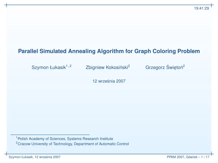
19:41:29 Parallel Simulated Annealing Algorithm for Graph Coloring Problem Grzegorz Szymon ukasik 1 , 2 nski 2 n 2 Zbigniew Kokosi Swi eto 12 wrze snia 2007 1 Polish Academy of Sciences, Systems Research Institute 2 Cracow
19:41:29 Parallel Simulated Annealing Algorithm for Graph Coloring Problem Grzegorz ´ Szymon Łukasik 1 , 2 nski 2 n 2 Zbigniew Kokosi´ Swi˛ eto´ 12 wrze´ snia 2007 1 Polish Academy of Sciences, Systems Research Institute 2 Cracow University of Technology, Department of Automatic Control Szymon Łukasik, 12 wrze´ snia 2007 PPAM 2007, Gda´ nsk – 1 / 17
19:41:29 Introduction • Graph Coloring Problem (GCP) • Parallel Simulated Annealing Parallel Simulated Annealing for GCP Experimental results Final remarks Introduction Szymon Łukasik, 12 wrze´ snia 2007 PPAM 2007, Gda´ nsk – 2 / 17
19:41:29 Graph Coloring Problem (GCP) Introduction Let: G = ( V, E ) be a given graph with n vertices V connected with m • Graph Coloring Problem (GCP) edges E • Parallel Simulated Annealing Graph Coloring Problem: Find an assignment of k colors to vertices Parallel Simulated Annealing c : V → { 1 , . . . , k } , k � n such as ∀ ( u, v ) ∈ E : c ( u ) � = c ( v ) and k is for GCP minimal (graph chromatic number χ ( G ) . Experimental results Final remarks GCP is one of the NP-hard problems. Main heuristic solving methods: local and tabu search (Galinier & Hertz, 2006), • genetic algorithms (Fleurent & Ferland, 1996), • simulated annealing (Johnson et al., 1991), • + one metaheuristics application - parallel genetic algorithm (Kokosi´ nski et al., 2005). Szymon Łukasik, 12 wrze´ snia 2007 PPAM 2007, Gda´ nsk – 3 / 17
19:41:29 Parallel Simulated Annealing Two main concepts (Lee & Lee, 1996): Introduction • Graph Coloring Problem a ) parallel moves (trials) - single Markov chain is being evaluated by (GCP) • Parallel Simulated multiple processing units calculating possible moves from one state to Annealing Parallel Simulated Annealing another, for GCP b ) multiple Markov chains - uses multiple threads for computing Experimental results independent chains of solutions and exchanging the obtained results Final remarks on a regular basis (synchronous or asynchronous). Recent years brought rapid development of this technique (both in theory and practice). Some applications and improvements are: vehicle routing (Czech, 2001), flow shop (Wodecki & Bo˙ zejko, 2001), • global optimization (Onba¸ soˇ glu & Özdamar, 2005) multisteps, backtrack jumps (Bo˙ zejko & Wodecki, 2004), genetic • algorithm at higher level (Tomoyuki et al., 2000). Szymon Łukasik, 12 wrze´ snia 2007 PPAM 2007, Gda´ nsk – 4 / 17
19:41:29 Introduction Parallel Simulated Annealing for GCP • Proposed Algorithm • Solution representation & Cost assessment • Neighborhood Generation - Algorithm Experimental results Final remarks Parallel Simulated Annealing for GCP Szymon Łukasik, 12 wrze´ snia 2007 PPAM 2007, Gda´ nsk – 5 / 17
19:41:29 Proposed Algorithm Introduction i f proc=master Parallel Simulated Annealing best_cost := i n f i n i t y ; i f for GCP proc=slave / / generate i n i t i a l s o l u t i o n randomly at each slave • Proposed Algorithm s o l u t i o n [ proc ] : = Generate_Initial_Solution ( ) ; • Solution representation & for iter_no do i t e r :=1 to Cost assessment i f proc=slave • Neighborhood Generation / / each slave generates a new s o l u t i o n - Algorithm neighbor_solution [ proc ] : = Generate_Neighbor_Sol( s o l u t i o n [ proc ] ) ; / / and accepts i t as a current one according to SA methodology Experimental results s o l u t i o n [ proc ] : = Anneal ( neighbor_solution [ proc ] , s o l u t i o n [ proc ] , T ) ; Final remarks / / a l l solutions are then gathered at master Gather_at_master ( s o l u t i o n [ proc ] ) ; i f proc=master current_cost := i n f i n i t y ; / / f i n d s o l u t i o n with minimum cost and set i t as a current one for slaves_no do j :=1 to i f Cost ( s o l u t i o n [ j ]) < current_cost current_solution := s o l u t i o n [ j ] ; current_cost := Cost ( s o l u t i o n [ j ] ) ; / / update best s o l u t i o n found ( i f applicable ) i f current_cost <best_cost best_solution := current_solution ; best_cost := current_cost ; / / i f stop condition f u l f i l l e d − end main loop i f best_cost <=target_cost break ; / / d i s t r i b u t e p e r i o d i c a l l y current s o l u t i o n among a l l slaves i f i t e r mod e_i = 0 s o l u t i o n [ proc ] : = D i s t r i b u t e ( current_solution ) ; / / update annealing temperature i f appropriate T:= Update_Temperature(T ) ; i f proc=master return best_solution ; Szymon Łukasik, 12 wrze´ snia 2007 PPAM 2007, Gda´ nsk – 6 / 17
19:41:29 Solution representation & Cost assessment A graph coloring c is represented by a sequence of natural numbers Introduction • Parallel Simulated Annealing c = < c [1] , . . . , c [ n ] > , c [ i ] ∈ { 1 , . . . , k } . for GCP • Proposed Algorithm Cost of solution is determined using following cost function (Kokosi´ nski • • Solution representation & Cost assessment et al., 2005): • Neighborhood Generation - Algorithm � f ( c ) = q ( u, v ) + d + k Experimental results ( u,v ) ∈ E Final remarks where q – is a penalty function: � 2 when c ( u ) = c ( v ) q ( u, v ) = 0 otherwise d – is a coefficient for solution with conflicts: � 1 when � ( u,v ) ∈ E q ( u, v ) > 0 d = 0 when � ( u,v ) ∈ E q ( u, v ) = 0 and k – is the number of colors used. Szymon Łukasik, 12 wrze´ snia 2007 PPAM 2007, Gda´ nsk – 7 / 17
19:41:29 Neighborhood Generation - Algorithm Introduction / / check f o r verti ces with color c o n f l i c t s Parallel Simulated Annealing for GCP c o n f l i c t _ v e r t i c e s := Find_Conflicting_Vertices ( c ) ; • Proposed Algorithm • Solution representation & Cost assessment i f sizeof ( c o n f l i c t _ v e r t i c e s )>0 do • Neighborhood Generation - Algorithm / / c o n f l i c t s were found − choose random c o n f l i c t i n g vertex Experimental results vertex_to_change :=random ( c o n f l i c t _ v e r t i c e s ) ; Final remarks / / and replace i t s color randomly / / with one of the colors {1 , . . . , k+1} c [ vertex_to_change ] : = random ( k +1); else / / i f no c o n f l i c t s are found choose random vertex vertex_to_change :=random ( n ) ; / / and replace i t s color randomly / / with one of the colors {1 , . . . , k } c [ vertex_to_change ] : = random ( k ) ; return c ; Szymon Łukasik, 12 wrze´ snia 2007 PPAM 2007, Gda´ nsk – 8 / 17
19:41:29 Introduction Parallel Simulated Annealing for GCP Experimental results • Testing environment • Simulated Annealing parameters settings • Parallel Simulated Annealing for GCP performance evaluation • Comparison with Parallel Genetic Algorithm Experimental results Final remarks Szymon Łukasik, 12 wrze´ snia 2007 PPAM 2007, Gda´ nsk – 9 / 17
19:41:29 Testing environment Introduction Algorithm was implemented using MPICH-2 library and tested on Parallel Simulated Annealing • for GCP LINUX-based system. Experimental results • Testing environment � Xeon TM machine using All experiments were carried out on one Intel R • • Simulated Annealing parameters settings simulated parallelism (number of iterations was inversely proportional to • Parallel Simulated Annealing for GCP the number of slaves). performance evaluation • Comparison with Parallel Genetic Algorithm As test instances standard DIMACS graphs were used. • Final remarks Initial temperature was determined from a pilot run consisting of 1% • (relative to overall iteration number) positive transitions. For experiments following values of SA control parameters were • chosen: α = 0 . 95 and β = 1 . 05 . The termination condition was either achieving the optimal solution or • the required number of iterations. Szymon Łukasik, 12 wrze´ snia 2007 PPAM 2007, Gda´ nsk – 10 / 17
19:41:29 Simulated Annealing parameters settings Introduction Parallel Simulated Annealing for GCP Experimental results P (∆ cost, 0) 1 2 3 Graph Tf k 0 • Testing environment G(V,E) Description Results Best P Results Best Tf Results Best k 0 • Simulated Annealing parameters settings anna, χ ( G ) = 11 best f(c) 11 . 12 70% 11 . 00 0 . 04 · T 0 11 . 12 χ ( G ) • Parallel Simulated | V | = 138 avg. f(c) 11 . 32 11 . 14 11 . 17 Annealing for GCP | E | = 493 σf ( c ) 0 . 29 0 . 21 0 . 05 performance evaluation • Comparison with Parallel queen8_8, χ ( G ) = 9 best f(c) 11 . 33 60% 10 . 60 0 . 06 · T 0 11 . 33 χ ( G ) Genetic Algorithm | V | = 64 avg. f(c) 11 . 46 11 . 84 11 . 41 | E | = 728 σf ( c ) 0 . 10 1 . 26 0 . 05 Final remarks mulsol.i.4, χ ( G ) = 31 best f(c) 38 . 23 80% 31 . 03 0 . 2 · T 0 37 . 63 χ ( G ) − 5 | V | = 197 avg. f(c) 38 . 66 33 . 65 38 . 22 | E | = 3925 σf ( c ) 0 . 46 1 . 64 0 . 36 myciel7, χ ( G ) = 8 best f(c) 12 . 95 60% 8 . 00 0 . 2 · T 0 11 . 38 χ ( G ) − 5 avg. f(c) | V | = 191 13 . 22 9 . 47 12 . 93 | E | = 2360 σf ( c ) 0 . 34 1 . 60 0 . 96 1 500 runs, iter _ no = 10000 , T f = 0 . 1 , k 0 = χ ( G ) 2 500 runs, iter _ no = 10000 , P (∆ cost, 0 ) = 70% , k 0 = χ ( G ) 3 500 runs, iter _ no = 10000 , P (∆ cost, 0 ) = 70% , T f = 0 . 05 · T 0 , Szymon Łukasik, 12 wrze´ snia 2007 PPAM 2007, Gda´ nsk – 11 / 17
Recommend
More recommend
Explore More Topics
Stay informed with curated content and fresh updates.
