Simulated Annealing G5BAIM: Artificial Intelligence Methods Graham - PowerPoint PPT Presentation
Simulated Annealing G5BAIM: Artificial Intelligence Methods Graham Kendall 15 Feb 09 1 Simulated Annealing G5BAIM Artificial Intelligence Methods Graham Kendall Simulated Annealing Simulated Annealing Simulated Annealing
Simulated Annealing G5BAIM: Artificial Intelligence Methods Graham Kendall 15 ‐ Feb ‐ 09 1
Simulated Annealing G5BAIM Artificial Intelligence Methods Graham Kendall Simulated Annealing
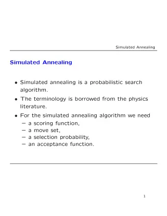
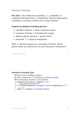
Simulated Annealing Simulated Annealing • Motivated by the physical annealing process • Material is heated and slowly cooled into a uniform structure • Simulated annealing mimics this process • The first SA algorithm was developed in 1953 (Metropolis)
Simulated Annealing Simulated Annealing • Compared to hill climbing the main difference is that SA allows downwards steps • Simulated annealing also differs from hill climbing in that a move is selected at random and then decides whether to accept it • In SA better moves are always accepted. Worse moves are not
Simulated Annealing Simulated Annealing • Kirkpatrick (1982) applied SA to optimisation problems • Kirkpatrick, S , Gelatt, C.D., Vecchi, M.P. 1983. Optimization by Simulated Annealing. Science, vol 220, No. 4598, pp 671- 680
Simulated Annealing The Problem with Hill Climbing • Gets stuck at local minima • Possible solutions • Try several runs, starting at different positions • Increase the size of the neighbourhood (e.g. in TSP try 3-opt rather than 2-opt)
Simulated Annealing To accept or not to accept? • The law of thermodynamics states that at temperature, t, the probability of an increase in energy of magnitude, δ E, is given by P( δ E) = exp(- δ E /kt) Where k is a constant known as Boltzmann’s constant •
Simulated Annealing To accept or not to accept - SA? P = exp( ‐ c/ t ) > r • Where • c is change in the evaluation function • t the current temperature • r is a random number between 0 and 1 Change in Change in Evaluation Temperature Evaluation Temperature Function of System exp(-C/T) Function of System exp(-C/T) 10 100 0.904837418 10 10 0.367879441 20 100 0.818730753 20 10 0.135335283 30 100 0.740818221 30 10 0.049787068 40 100 0.670320046 40 10 0.018315639 50 100 0.60653066 50 10 0.006737947 60 100 0.548811636 60 10 0.002478752 70 100 0.496585304 70 10 0.000911882 80 100 0.449328964 80 10 0.000335463 90 100 0.40656966 90 10 0.00012341 100 100 0.367879441 100 10 4.53999E-05 110 100 0.332871084 110 10 1.67017E-05 120 100 0.301194212 120 10 6.14421E-06 130 100 0.272531793 130 10 2.26033E-06 140 100 0.246596964 140 10 8.31529E-07 • Example 150 100 0.22313016 150 10 3.05902E-07 160 100 0.201896518 160 10 1.12535E-07 170 100 0.182683524 170 10 4.13994E-08 180 100 0.165298888 180 10 1.523E-08 190 100 0.149568619 190 10 5.6028E-09 200 100 0.135335283 200 10 2.06115E-09
Simulated Annealing To accept or not to accept - SA? Change Temp exp(-C/T) Change Temp exp(-C/T) 0.2 0.95 0.810157735 0.2 0.1 0.135335283 0.4 0.95 0.656355555 0.4 0.1 0.018315639 0.6 0.95 0.53175153 0.6 0.1 0.002478752 0.8 0.95 0.430802615 0.8 0.1 0.000335463
Simulated Annealing To accept or not to accept - SA? • The probability of accepting a worse state is a function of both the temperature of the system and the change in the cost function • As the temperature decreases, the probability of accepting worse moves decreases • If t =0, no worse moves are accepted (i.e. hill climbing)
Simulated Annealing SA Algorithm • The most common way of implementing an SA algorithm is to implement hill climbing with an accept function and modify it for SA • The example shown here is taken from Russell/Norvig
Simulated Annealing SA Algorithm - 1 Function SIMULATED-ANNEALING(Problem, Schedule) returns a solution state Inputs: Problem, a problem Schedule, a mapping from time to temperature Local Variables : Current, a node Next, a node T , a “temperature” controlling the probability of downward steps Current = MAKE-NODE(INITIAL-STATE[Problem]) For t = 1 to ∞ do T = Schedule[ t ] If T = 0 then return Current Next = a randomly selected successor of Current Λ E = VALUE[Next] – VALUE[Current] if Λ E > 0 then Current = Next else Current = Next only with probability exp(- Λ E/T)
Simulated Annealing SA Algorithm - Observations • The cooling schedule is hidden in this algorithm - but it is important (more later) • The algorithm assumes that annealing will continue until temperature is zero - this is not necessarily the case
Simulated Annealing SA Algorithm - 2 procedure SIMULATED ANNEALING; begin INITIALIZE ( istart , c0, L0); k := 0; i := i start ; repeat for l := 1 to L k do begin GENERATE ( j from S i ); if f ( j ) ≤ f (i ) then i := j else if exp ( f (i) − f ( j )) / ck > random[0, 1) then i := j end; k := k + 1; CALCULATE LENGTH (L k ); CALCULATE CONTROL (c k ); until stopcriterion end;
Simulated Annealing SA Algorithm - 2 procedure SIMULATED ANNEALING; begin INITIALIZE computes a start INITIALIZE ( i start , c 0 , L 0 ); solution and initial values of the k := 0; parameters c and L; i := i start ; repeat for l := 1 to L k do begin GENERATE ( j from S i ); if f ( j ) ≤ f (i ) then i := j else if exp ( f (i) − f ( j )) / ck > random[0, 1) then i := j end; k := k + 1; CALCULATE LENGTH (L k ); CALCULATE CONTROL (c k ); until stopcriterion end;
Simulated Annealing SA Algorithm - 2 procedure SIMULATED ANNEALING; begin INITIALIZE ( istart , c0, L0); k := 0; i := i start ; repeat for l := 1 to L k do GENERATE selects a solution begin from the neighborhood of the GENERATE ( j from S i ); current solution; if f ( j ) ≤ f (i ) then i := j else if exp ( f (i) − f ( j )) / ck > random[0, 1) then i := j end; k := k + 1; CALCULATE LENGTH (L k ); CALCULATE CONTROL (c k ); until stopcriterion end;
Simulated Annealing SA Algorithm - 2 procedure SIMULATED ANNEALING; begin INITIALIZE ( istart , c0, L0); k := 0; i := i start ; repeat for l := 1 to L k do begin GENERATE ( j from S i ); if f ( j ) ≤ f (i ) then i := j else if exp ( f (i) − f ( j )) / ck > random[0, 1) then i := j end; CALCULATE LENGTH and k := k + 1; CALCULATE CONTROL compute CALCULATE LENGTH (L k ); CALCULATE CONTROL (c k ); new values for the parameters L and c, until stopcriterion respectively end;
Simulated Annealing SA Cooling Schedule Starting Temperature • Final Temperature • Temperature Decrement • Iterations at each temperature •
Simulated Annealing SA Cooling Schedule - Starting Temperature Starting Temperature • • Must be hot enough to allow moves to almost neighbourhood state (else we are in danger of implementing hill climbing) • Must not be so hot that we conduct a random search for a period of time • Problem is finding a suitable starting temperature
Simulated Annealing SA Cooling Schedule - Starting Temperature Starting Temperature - Choosing • • If we know the maximum change in the cost function we can use this to estimate • Start high, reduce quickly until about 60% of worse moves are accepted. Use this as the starting temperature • Heat rapidly until a certain percentage are accepted the start cooling
Simulated Annealing SA Cooling Schedule - Final Temperature Final Temperature - Choosing • • It is usual to let the temperature decrease until it reaches zero However, this can make the algorithm run for a lot longer, especially when a geometric cooling schedule is being used • In practise, it is not necessary to let the temperature reach zero because the chances of accepting a worse move are almost the same as the temperature being equal to zero
Simulated Annealing SA Cooling Schedule - Final Temperature Final Temperature - Choosing • • Therefore, the stopping criteria can either be a suitably low temperature or when the system is “frozen” at the current temperature (i.e. no better or worse moves are being accepted)
Simulated Annealing SA Cooling Schedule - Temperature Decrement Temperature Decrement • • Theory states that we should allow enough iterations at each temperature so that the system stabilises at that temperature • Unfortunately, theory also states that the number of iterations at each temperature to achieve this might be exponential to the problem size
Simulated Annealing SA Cooling Schedule - Temperature Decrement Temperature Decrement • • We need to compromise • We can either do this by doing a large number of iterations at a few temperatures, a small number of iterations at many temperatures or a balance between the two
Simulated Annealing SA Cooling Schedule - Temperature Decrement Temperature Decrement • – Linear • temp = temp - x – Geometric • temp = temp * x • Experience has shown that α should be between 0.8 and 0.99, with better results being found in the higher end of the range. Of course, the higher the value of α , the longer it will take to decrement the temperature to the stopping criterion
Simulated Annealing SA Cooling Schedule - Iterations Iterations at each temperature • – A constant number of iterations at each temperature – Another method, first suggested by (Lundy, 1986) is to only do one iteration at each temperature, but to decrease the temperature very slowly.
Recommend
More recommend
Explore More Topics
Stay informed with curated content and fresh updates.
