Pandas Data Manipulation in Python 1 / 31 Pandas Built on NumPy - PowerPoint PPT Presentation
Pandas Data Manipulation in Python 1 / 31 Pandas Built on NumPy Adds data structures and data manipulation tools Enables easier data cleaning and analysis 1 import pandas as pd 2 pd.set_option("display.width", 120) That
Pandas Data Manipulation in Python 1 / 31
Pandas ◮ Built on NumPy ◮ Adds data structures and data manipulation tools ◮ Enables easier data cleaning and analysis 1 import pandas as pd 2 pd.set_option("display.width", 120) That last line allows you to display DataFrames with many columns without wrapping. 2 / 31
Pandas Fundamentals Three fundamental Pandas data structures: ◮ Series - a one-dimensional array of values indexed by a pd.Index ◮ Index - an array-like object used to access elements of a Series or DataFrame ◮ DataFrame - a two-dimensional array with flexible row indices and column names 3 / 31
Series from List 1 In [4]: data = pd.Series(['a','b','c','d']) 2 3 In [5]: data 4 Out[5]: 5 0 a 6 1 b 7 2 c 8 3 d 9 dtype: object The 0..3 in the left column are the pd.Index for data : 1 In [7]: data.index 2 Out[7]: RangeIndex(start=0, stop=4, step=1) The elements from the Python list we passed to the pd.Series constructor make up the values: 1 In [8]: data.values 2 Out[8]: array(['a', 'b', 'c', 'd'], dtype=object) Notice that the values are stored in a Numpy array. 4 / 31
Series from Sequence You can construct a list from any definite sequence: 1 In [24]: pd.Series(np.loadtxt('exam1grades.txt')) 2 Out[24]: 3 0 72.0 4 1 72.0 5 2 50.0 6 ... 7 134 87.0 8 dtype: float64 or 1 In [25]: pd.Series(open('exam1grades.txt').readlines()) 2 Out[25]: 3 0 72\n 4 1 72\n 5 2 50\n 6 ... 7 134 87\n 8 dtype: object . . . but not an indefinite sequence: 1 In [26]: pd.Series(open('exam1grades.txt')) 2 ... 3 TypeError: object of type '_io.TextIOWrapper' has no len() 5 / 31
Series from Dictionary 1 salary = {"Data Scientist": 110000, 2 "DevOps Engineer": 110000, 3 "Data Engineer": 106000, 4 "Analytics Manager": 112000, 5 "Database Administrator": 93000, 6 "Software Architect": 125000, 7 "Software Engineer": 101000, 8 "Supply Chain Manager": 100000} Create a pd.Series from a dict : 1 In [14]: salary_data = pd.Series(salary) 2 3 In [15]: salary_data 4 Out[15]: 5 Analytics Manager 112000 6 Data Engineer 106000 7 Data Scientist 110000 8 Database Administrator 93000 9 DevOps Engineer 110000 10 Software Architect 125000 11 Software Engineer 101000 12 Supply Chain Manager 100000 13 dtype: int64 The index is a sorted sequence of the keys of the dictionary passed 6 / 31 to
Series with Custom Index General form of Series constructor is pd.Series(data, index=index) ◮ Default is integer sequence for sequence data and sorted keys of dictionaries ◮ Can provide a custom index: 1 In [29]: pd.Series([1,2,3], index=['a', 'b', 'c']) 2 Out[29]: 3 a 1 4 b 2 5 c 3 6 dtype: int64 The index object itself is an immutable array with set operations. 1 In [30]: i1 = pd.Index([1,2,3,4]) 2 3 In [31]: i2 = pd.Index([3,4,5,6]) 4 5 In [32]: i1[1:3] 6 Out[32]: Int64Index([2, 3], dtype='int64') 7 8 In [33]: i1 & i2 # intersection 9 Out[33]: Int64Index([3, 4], dtype='int64') 10 7 / 31 11 In [34]: i1 | i2 # union 12
Series Indexing and Slicing Indexing feels like dictionary access due to flexible index objects: 1 In [37]: data = pd.Series(['a', 'b', 'c', 'd']) 2 3 In [38]: data[0] 4 Out[38]: 'a' 5 6 In [39]: salary_data['Software Engineer'] 7 Out[39]: 101000 But you can also slice using these flexible indices: 1 In [40]: salary_data['Data Scientist':'Software Engineer'] 2 Out[40]: 3 Data Scientist 110000 4 Database Administrator 93000 5 DevOps Engineer 110000 6 Software Architect 125000 7 Software Engineer 101000 8 dtype: int64 8 / 31
Basic DataFrame Structure A DataFrame is a series Serieses with the same keys. For example, consider the following dictionary of dictionaries meant to leverage your experience with spreadsheets (in spreadsheet.py): 1 In [5]: import spreadsheet; spreadsheet.cells 2 3 Out[5]: 4 {'A': {1: 'A1', 2: 'A2', 3: 'A3'}, 5 'B': {1: 'B1', 2: 'B2', 3: 'B3'}, 6 'C': {1: 'C1', 2: 'C2', 3: 'C3'}, 7 'D': {1: 'D1', 2: 'D2', 3: 'D3'}} All of these dictionaries have the same keys, so we can pass this dictionary of dictionaries to the DataFrame constructor: 1 In [7]: ss = pd.DataFrame(spreadsheet.cells); ss 2 3 Out[7]: 4 A B C D 5 1 A1 B1 C1 D1 6 2 A2 B2 C2 D2 7 3 A3 B3 C3 D3 9 / 31
Basic DataFrame Structure 1 In [5]: import spreadsheet; spreadsheet.cells 2 3 Out[5]: 4 {'A': {1: 'A1', 2: 'A2', 3: 'A3'}, 5 'B': {1: 'B1', 2: 'B2', 3: 'B3'}, 6 'C': {1: 'C1', 2: 'C2', 3: 'C3'}, 7 'D': {1: 'D1', 2: 'D2', 3: 'D3'}} All of these dictionaries have the same keys, so we can pass this dictionary of dictionaries to the DataFrame constructor: 1 In [7]: ss = pd.DataFrame(spreadsheet.cells); ss 2 3 Out[7]: 4 A B C D 5 1 A1 B1 C1 D1 6 2 A2 B2 C2 D2 7 3 A3 B3 C3 D3 ◮ Each column is a Series whose keys (index) are the values printed to the left (1, 2 and 3). ◮ Each row is a Series whose keys (index) are the column headers. Try evaluating ss.columns and ss.index . 10 / 31
DataFrame Example Download hotjobs.py and do a %load hotjobs.py (to evaluate the code in the top-level namespace instead of importing it). 1 In [42]: jobs = pd.DataFrame({'salary': salary, 'openings': openings}) 2 3 In [43]: jobs 4 Out[43]: 5 openings salary 6 Analytics Manager 1958 112000 7 Data Engineer 2599 106000 8 Data Scientist 4184 110000 9 Database Administrator 2877 93000 10 DevOps Engineer 2725 110000 11 Software Architect 2232 125000 12 Software Engineer 17085 101000 13 Supply Chain Manager 1270 100000 14 UX Designer 1691 92500 1 In [46]: jobs.index 2 Out[46]: 3 Index(['Analytics Manager', 'Data Engineer', 'Data Scientist', 4 'Database Administrator', 'DevOps Engineer', 'Software Architect', 5 'Software Engineer', 'Supply Chain Manager', 'UX Designer'], 6 dtype='object') 7 8 In [47]: jobs.columns 11 / 31 9 Out[47]: Index(['openings', 'salary'], dtype='object')
Simple DataFrame Indexing Simplest indexing of DataFrame is by column name. 1 In [48]: jobs['salary'] 2 Out[48]: 3 Analytics Manager 112000 4 Data Engineer 106000 5 Data Scientist 110000 6 Database Administrator 93000 7 DevOps Engineer 110000 8 Software Architect 125000 9 Software Engineer 101000 10 Supply Chain Manager 100000 11 UX Designer 92500 12 Name: salary, dtype: int64 Each colum is a Series: 1 In [49]: type(jobs['salary']) 2 Out[49]: pandas.core.series.Series 12 / 31
General Row Indexing The loc indexer indexes by row name: 1 In [13]: jobs.loc['Software Engineer'] 2 Out[13]: 3 openings 17085 4 salary 101000 5 Name: Software Engineer, dtype: int64 6 7 In [14]: jobs.loc['Data Engineer':'Databse Administrator'] 8 Out[14]: 9 openings salary 10 Data Engineer 2599 106000 11 Data Scientist 4184 110000 12 Database Administrator 2877 93000 Note that slice ending is inclusive when indexing by name. The iloc indexer indexes rows by position: 1 In [15]: jobs.iloc[1:3] 2 Out[15]: 3 openings salary 4 Data Engineer 2599 106000 5 Data Scientist 4184 110000 Note that slice ending is exclusive when indexing by integer position. 13 / 31
Special Case Row Indexing 1 In [16]: jobs[:2] 2 Out[16]: 3 openings salary 4 Analytics Manager 1958 112000 5 Data Engineer 2599 106000 6 7 In [17]: jobs[jobs['salary'] > 100000] 8 Out[17]: 9 openings salary 10 Analytics Manager 1958 112000 11 Data Engineer 2599 106000 12 Data Scientist 4184 110000 13 DevOps Engineer 2725 110000 14 Software Architect 2232 125000 15 Software Engineer 17085 101000 Try jobs['salary'] > 100000 by itself. What’s happening in In[17] above? 14 / 31
loc and iloc Indexing The previous examples are shortcuts for loc and iloc indexing: 1 In [20]: jobs.iloc[:2] 2 Out[20]: 3 openings salary 4 Analytics Manager 1958 112000 5 Data Engineer 2599 106000 6 7 In [21]: jobs.loc[jobs['salary'] > 100000] 8 Out[21]: 9 openings salary 10 Analytics Manager 1958 112000 11 Data Engineer 2599 106000 12 Data Scientist 4184 110000 13 DevOps Engineer 2725 110000 14 Software Architect 2232 125000 15 Software Engineer 17085 101000 15 / 31
Aggregate Functions The values in a series is a numpy.ndarray , so you can use NumPy functions, broadcasting, etc. ◮ Average salary for all these jobs: 1 In [14]: np.average(jobs['salary']) 2 Out[14]: 107125.0 ◮ Total number of openings: 1 In [15]: np.sum(jobs['openings']) 2 Out[15]: 34930 And so on. 16 / 31
Adding Columns by Broadcasting Add column by broadcasting a constant value: 1 In [16]: jobs['DM Prepares'] = True 2 3 In [17]: jobs 4 Out[17]: 5 openings salary DM Prepares 6 Analytics Manager 1958 112000 True 7 Data Engineer 2599 106000 True 8 Data Scientist 4184 110000 True 9 Database Administrator 2877 93000 True 10 DevOps Engineer 2725 110000 True 11 Software Architect 2232 125000 True 12 Software Engineer 17085 101000 True 13 Supply Chain Manager 1270 100000 True 17 / 31
Recommend
More recommend
Explore More Topics
Stay informed with curated content and fresh updates.
![Merging DataFrames Merging DataFrames with pandas Population DataFrame In [1]: import pandas as](https://c.sambuz.com/751912/merging-dataframes-s.webp)



![Whats new and awesome in pandas pandas? In [13]: foo Out[13]: methyl1 age edu](https://c.sambuz.com/777840/what-s-new-and-awesome-in-pandas-pandas-s.webp)

