Pairwise alignment using HMMs - Ch.4 Durbin et al. Recall the - PowerPoint PPT Presentation
1 Pairwise alignment using HMMs - Ch.4 Durbin et al. Recall the Needleman-Wunsch algorithm for affine gap penalty: V M ( i 1 , j 1) V M ( i, j ) = s ( x i , y j ) + max V X ( i 1 , j 1) V Y ( i 1 , j
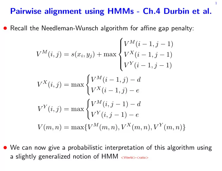
1 Pairwise alignment using HMMs - Ch.4 Durbin et al. • Recall the Needleman-Wunsch algorithm for affine gap penalty: V M ( i − 1 , j − 1) V M ( i, j ) = s ( x i , y j ) + max V X ( i − 1 , j − 1) V Y ( i − 1 , j − 1) � V M ( i − 1 , j ) − d V X ( i, j ) = max V X ( i − 1 , j ) − e � V M ( i, j − 1) − d V Y ( i, j ) = max V Y ( i, j − 1) − e V ( m, n ) = max { V M ( m, n ) , V X ( m, n ) , V Y ( m, n ) } • We can now give a probabilistic interpretation of this algorithm using a slightly generalized notion of HMM < Viterbi >< ratio >
2 “Pair HMMs” • A pair HMM generates an alignment by simultaneously producing two sequences of symbols • The M (match) state emits a pair of symbols, one for each sequence: ( x i , y j ) ∼ p ( x i , y j ) • The X ( x -insertion) state emits only an “ X symbol”: x i ∼ q ( x i ) • The Y ( y -insertion) state emits only a “ Y symbol”: y j ∼ q ( y j )
3 Pair HMM - cont. • The model above does not generate a probability distribution over all possible sequences • for that we need to add Begin and End states: • The expected length of the generated alignment is 1 τ • The transitions of the Markov chain are given by p MM = p BM = 1 − 2 δ − τ , p MX = p MY = δ , p XX = ε , p XM = 1 − ε − δ , etc.
4 Most probable alignment • We can only observe x and y : unlike in HMMs we cannot observe the joint emission from the M state • Let S ij be the set of paths s compatible with an alignment of x 1: i and y 1: j • i.e. the path visits states { M, X } exatly i times and states { M, Y } exatly j times • Given the observed sequences x and y , S mn is in 1:1 correspondence with the set of alignments of x and y • The advantage of the pair HMM framework is now we can ask for the most probable alignment given the data • same as maximizing p ( x , y , s ) over the path s
5 Most probable alignment - cont. • For α ∈ { M, X, Y } let v α ( i, j ) = s ∈S ij : s ( | s | )= α p ( x 1: i , y 1: j , s 1: | s | ) , max where | s | is the length of the alignment of s . • Clearly, p ( x , y , s ) = max { v M ( m, n ) , v X ( m, n ) , v Y ( m, n ) } · τ max s • note that the rhs is in fact v E ( m, n ) • The following claim shows how to recursively compute v α ( i, j )
6 Viterbi for pair HMM • Claim. For m ≥ i ≥ 0 , n ≥ j ≥ 0 with i + j > 0 : p MM · v M ( i − 1 , j − 1) v M ( i, j ) = p ( x i , y j ) · max p XM · v X ( i − 1 , j − 1) p Y M · v Y ( i − 1 , j − 1) � p MX · v M ( i − 1 , j ) v X ( i, j ) = q ( x i ) · max p XX · v X ( i − 1 , j ) � p MY · v M ( i, j − 1) v Y ( i, j ) = q ( y j ) · max p Y Y · v Y ( i, j − 1) where v • ( i, − 1) = v • ( − 1 , j ) = v [ XY ] (0 , 0) = 0 , and v M (0 , 0) := 1 • v M (0 , 0) is in fact a surrogate for v B (0 , 0) < Needleman-Wunsch >< ratio >
7 Viterbi for pair HMM - cont. • This algorithm is similar but still differs from Needleman-Wunsch • logarithms should be used • log-odds rather than log-odds are computed ratio (BLOSUM/PAM) • The following random model simply dumps the symbols of x and the y without any correlation (no match states) m n p R ( x , y ) = η (1 − η ) m q ( x i ) η (1 − η ) n � � q ( y j ) i =1 j =1
8 Viterbi for maximal log-odds ratio • Look for the path s that maximizes the log-odds ratio log p M ( s , x , y ) p R ( s , x , y ) p M ( x 1: i , y 1: j , s 1: | s | ) • Let V α ( i, j ) = max s ∈S ij : s ( | s | )= α log p R ( x 1: i , y 1: j , s 1: | s | ) • Analogously to the log-odds case we have log p MM (1 − η ) 2 + V M ( i − 1 , j − 1) V M ( i, j ) = log p ( x i , y j ) p XM (1 − η ) 2 + V X ( i − 1 , j − 1) log q ( x i ) q ( y j ) + max (1 − η ) 2 + V Y ( i − 1 , j − 1) p Y M log � log p MX 1 − η + V M ( i − 1 , j ) V X ( i, j ) = log q ( x i ) q ( x i ) + max log p XX 1 − η + V X ( i − 1 , j ) � log p MY 1 − η + V M ( i, j − 1) V Y ( i, j ) = log q ( y j ) q ( y j ) + max < Needleman-Wunsch > 1 − η + V Y ( i, j − 1) log p Y Y
9 Viterbi as Needleman-Wunsch • To see the equivalence more clearly it is convenient to introduce s ( a, b ) = log p ( a, b ) p MM q ( a ) q ( b ) + log (1 − η ) 2 − d = log p MX/Y (1 − η ) + log p X/Y M p MM − e = log p XX/Y Y 1 − η • s ( a, b ) “assumes” we come from M p X/Y M • d “pre-corrects” that by adding c := log p MM • Only η 2 and the transitions from X/Y to E are left unbalanced: V M (0 , 0) := − 2 log η V E ( m, n ) := max { V M ( m, n ) , V X ( m, n ) − c, V Y ( m, n ) − c }
10 pair HMM for local alignment • As before we can look for optimal log-odds or log-odds ratio paths (the latter case will yield Smith-Waterman)
11 The likelihood that x and y are aligned • While it is interesting to note that the Needleman-Wunsch algorithm can be cast in the language of HMM • The real power of the HMM framework is that it allows us to answer questions such as • what is the likelihood that x and y are aligned, i.e., that they were generated by the model? • The answer is the probability that x , y will be generated by the model p ( x , y ) = � s p ( x , y , s ) • An analogue of the forward algorithm computes that: let f α ( i, j ) := P ( X 1: i = x 1: i , Y 1: j = y 1: j , S ( τ ij ) = α ) , where k k � � τ ij := min { k : 1 S ( l ) ∈{ M,X } = i and 1 S ( l ) ∈{ M,Y } = j } l =1 l =1
12 The likelihood that x and y are aligned - cont. • Claim. With the initial conditions f M (0 , 0) = 1 f [ XY ] (0 , 0) = 0 f • ( i, − 1) = f • ( − 1 , j ) = 0 , for i ≥ 0 , j ≥ 0 with i + j > 0 : f M ( i, j ) = p ( x i , y j )[ p MM · f M ( i − 1 , j − 1) + p XM · f X ( i − 1 , j − 1) + p Y M · f Y ( i − 1 , j − 1)] f X ( i, j ) = q ( x i )[ p MX · f M ( i − 1 , j ) + p XX · f X ( i − 1 , j )] f Y ( i, j ) = q ( y j )[ p MY · f M ( i, j − 1) + p Y Y · f Y ( i, j − 1)] , and p ( x , y ) = f E ( m, n ) = τ [ f M ( m, n ) + f X ( m, n ) + f Y ( m, n )]
13 Posterior distribution of an alignment • With p ( x , y ) we can find the posterior distribution of any particular alignment s : p ( s | x , y ) = p ( x , y , s ) p ( x , y ) • In particular we can apply it for s ∗ , the Viterbi solution • The answer is typically depressingly small ⊲ For example in the alpha globing vs. leghemoglobin case: ⊲ p ( s ∗ | x , y ) = 4 . 6 × 10 − 6
14 Sampling from the posterior distribution • Given the poor posterior probability of the Viterbi alignment • are there parts of the alignment which we are more confident of? • can we estimate posterior expectation of functionals of the align- ment as in posterior decoding? • We can do that through MC sampling from the posterior distribution • backward sampling (using forward algorithm) • forward sampling (using backward algorithm)
15 The backward algorithm • Analogously to the backward function for HMMs we define b α ( i, j ) := P ( X i +1: m = x i +1: m , Y j +1: n = y j +1: n , S ( τ ij ) = α ) , where k k � � τ ij := min { k : 1 S ( l ) ∈{ M,X } = i and 1 S ( l ) ∈{ M,Y } = j } l =1 l =1 • Durbin et al.: • as before we can add b M (0 , 0) as a surrogate for b B (0 , 0)
16 Forward posterior sampling (backward algorithm) • Inductively draw from the posterior distribution as follows: • start at state B with ( i, j ) := (0 , 0) • while ( i, j ) � = ( m, n ) : ⊲ given our hitherto path s ∈ S ( i, j ) randomly choose our next state α according to P [ S ( | s | + 1) = α | x , y , s ] ⊲ update: s = s ∧ α , and ( i, j ) := ( i + ( α ) , j + ( α )) := ( i + 1 α ∈{ M,X } , j + 1 α ∈{ M,Y } ) • output the resulting s ∈ S ( m, n ) (why is s ∈ S ( m, n ) ?) • Claim. The probability that we draw a path s ∈ S ( m, n ) is p ( s | x , y ) • Proof. To simplify notations assume s (0) = B does not count toward | s | . Then | s | � p ( s | x , y ) = p ( s ( i ) | x , y , s 0: i − 1 ) i =1
17 Forward posterior sampling - cont. • The algorithm hinges on finding P [ S ( | s | + 1) = α | x , y , s ] = p ( s ∧ α, x , y ) p ( s , x , y ) • Using the properties of the HMM we have: p ( s ∧ α, x , y ) = p ( x 1: i , y 1: j , s ) × P [ S ( | s | + 1) = α, x ( i + ( α )) , y ( j + ( α )) | x i , y j , s ] × p [ x i + ( α )+1: m , y j + ( α )+1: n | S ( | s | + 1) = α ] P [ S ( | s | + 1) = α, x ( i + ( α )) , y ( j + ( α )) | x i , y j , s ] p s ( | s | ) ,M · p ( x ( i + 1) , y ( j + 1)) α = M = p s ( | s | ) ,X · q ( x ( i + 1)) α = X p s ( | s | ) ,Y · q ( y ( j + 1)) α = Y
18 • Note that p [ x i + ( α )+1: m , y j + ( α )+1: n | S ( | s | + 1) = α ] = b α ( i + ( α ) , j + ( α )) • Finally, p ( s , x , y ) = p ( x 1: i , y 1: j , s ) p ( x i +1: m , y j +1: n | s ) = p ( x 1: i , y 1: j , s ) b s ( | s | ) ( i, j ) Thus, P [ S ( | s | + 1) = α | x , y , s ] = b α ( i + ( α ) , j + ( α )) b s ( | s | ) ( i, j ) p s ( | s | ) ,M · p ( x ( i + 1) , y ( j + 1)) α = M × p s ( | s | ) ,X · q ( x ( i + 1)) α = X p s ( | s | ) ,Y · q ( y ( j + 1)) α = Y
Recommend


More recommend
Explore More Topics
Stay informed with curated content and fresh updates.