Overview THE ATMOSPHERE Constituents Structure ATMOSPHERIC - PDF document

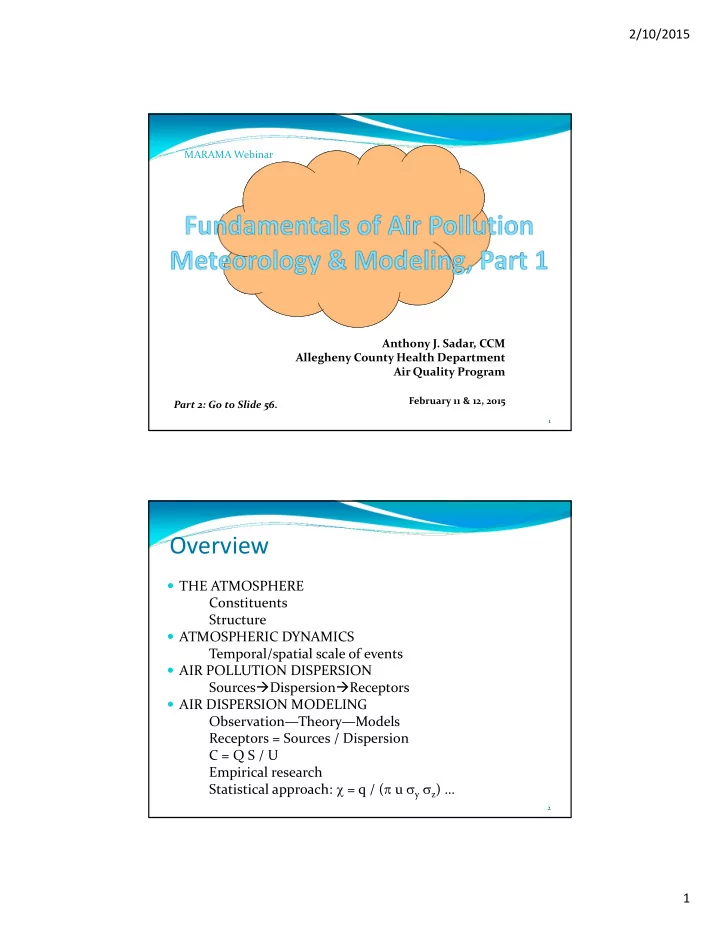
2/10/2015 MARAMA Webinar Anthony J. Sadar, CCM Allegheny County Health Department Air Quality Program February 11 & 12, 2015 Part 2: Go to Slide 56. 1 Overview  THE ATMOSPHERE Constituents Structure  ATMOSPHERIC DYNAMICS Temporal/spatial scale of events  AIR POLLUTION DISPERSION Sources  Dispersion  Receptors  AIR DISPERSION MODELING Observation—Theory—Models Receptors = Sources / Dispersion C = Q S / U Empirical research Statistical approach:  = q / (  u  y  z ) … 2 1

2/10/2015 Overview ( Continued )  US EPA GUIDELINES Guideline on Air Quality Models (Revised) , Appdx. W Other guidance/clarification  AERMOD & AERSCREEN Input requirements Output examples Interpretation of results Comparison between AERMOD and AERSCREEN  ADDITIONAL MODELS & APPLICATIONS Requirements for regulatory modeling 3 The Atmosphere  Constituents  Structure 4 2

2/10/2015 Constituents Permanent Percent Nitrogen (N2) 78.1 Oxygen (O2) 20.9 Argon (Ar) 0.9 Neon (Ne) 0.002 Variable Water Vapor (H2O) 0 ‐ 4 Carbon Dioxide (CO2) 0.04 Helium (He) 0.0005 Methane (CH4) 0.0002 Krypton (Kr) 0.0001 5 Structure Temperature changes with increasing altitude in atmosphere. ]- ABL Not to Scale. 6 3

2/10/2015 Atmospheric Boundary Layer (ABL)  Bottom layer of troposphere starting at earth’s surface and extending to several km during sunny afternoons.  Structure and height of ABL varies diurnally, during fair weather over land:  From tens of meters on mornings with a strong surface temperature inversion (when temperature increases with altitude) to several kilometers during sunny afternoons. 7 Atmospheric Dynamics  Temporal/Spatial Scales of Events Source: A World of Weather: Fundamentals of Meteorology , 4 th Edition, by Lee Grenci, Jon Nese, and David Babb, 2008, Figure 1.9. 8 4

2/10/2015 Conditions of Note  Topography  “Heat Island” Effect (Urban/Rural)  Land/Water (Diurnal “Sea Breeze”/“Land Breeze”)  Mountain/Valley (Diurnal Effects and Channeling)  Elevation 9 Conditions of Note ( Continued )  Overview Source: D. Carruthers, Chpt. 10, “Atmospheric Dispersion and Air Pollution Meteorology,” in Handbook of Atmospheric Science: Principles and Applications , C.N. Hewitt and A.V. Jackson, Editors, 2003. 10 5

2/10/2015 Conditions of Note ( Continued )  Topography Source: D. Carruthers, Chpt. 10, “Atmospheric Dispersion and Air Pollution Meteorology,” in Handbook of Atmospheric Science: Principles and Applications , C.N. Hewitt and A.V. Jackson, Editors, 2003. 11 Poll Question #1  The Heat Island Effect occurs in the Atmospheric Boundary Layer (True/False) 12 6

2/10/2015 Poll Question #2  Turbulence is a meso ‐ scale temporal event. (True/False) 13 Air Pollution Dispersion  Transport and Diffusion of Air Pollution  Sources  Dispersion  Receptors 14 7

2/10/2015 Air Dispersion Modeling • What is Modeling? • Modeling Components: ‐ Source considerations ‐ Dispersion considerations ‐ Receptor considerations 15 What Is Modeling?  A scientific “ model ” is a tentative representation of an observation based on interpretation of available information; a tool used to simulate real ‐ world conditions.  “ Air ‐ dispersion modeling ,” as described by the EPA, “uses mathematical formulations to characterize atmospheric processes that disperse a pollutant emitted by a source. Based on emissions and meteorological inputs, a dispersion model can be used to predict concentrations at selected downwind receptor locations.”  Note that “verification of the truth of any model is an impossible task” (ASTM International, D6589–05, 2010).  Models contain assumptions and limitations. 16 8

2/10/2015 What Is Modeling? (Continued) Observation Theory Models Adapted from: Numerical Weather and Climate Prediction , T. T. Warner, 2011, Fig. 1.1, p. 3. 17 Modeling Components Sources  Dispersion  Receptors 18 9

2/10/2015 Whence Highest Concentrations?  Large Emission Rate  Low Plume Rise  Overlapping Plumes  Stack ‐ Tip Downwash  Building ‐ Induced Downwash  Building Cavity 19 Whence Highest Conc.? ( Continued )  Proximity to Source(s)  Terrain ‐ Induced Downwash and Channeling  High Terrain  Short Ground Cover  Stable/Stagnant Atmosphere  Steady Wind Direction from Source(s) to Receptor(s) 20 10

2/10/2015 Source Considerations  “Worst ‐ case” conditions for emissions:  Maximum particle/gas discharge  Lowest release height  Lowest in ‐ vent/in ‐ stack temperature  Lowest exit gas velocity  Shortest distance to property line 21 Dispersion Considerations  “Worst ‐ case” meteorology:  No precipitation  Light winds from source to critical receptor(s)  Strong ground ‐ based temperature inversion (elevated inversion can also cause problems) Note: Wind Direction is direction from which wind is blowing. 22 11

2/10/2015 Receptor Considerations  “Worst ‐ case” conditions for receptors:  Closest, highest off ‐ site location  Plume centerline concentrations  Elevated receptor for malodor investigations 23 Simple Relationship  Sources  Dispersion  Receptors  Receptors = Sources / Dispersion R = S / D or 24 12

2/10/2015 Simple Dispersion Formula C = Q x S U Where, C is pollutant concentration (g/m 3 ) Q is rate of emissions exiting source (g/s) S is stability of atmosphere (m ‐ 2 ) U is horizontal wind speed (m/s) 25 How Does Emission Rate Affect C? 26 13

2/10/2015 How Does Wind Speed Affect C? 27 Poll Question #3  All else being equal, a pollutant concentration at a receptor will be higher with a higher stack.(True/False) 28 14

2/10/2015 Poll Question #4  All else being equal, a pollutant concentration at a receptor will be lower at low wind speed.(True/False) 29 How Does Stability Affect C? 30 15

2/10/2015 Stability Conditions  Traditionally, stability of lower atmosphere has been delineated as: 31 How Does Stability Affect Plumes? Smokestack emissions that continuously exhaust to the ambient air are referred to as “ plumes .” Plumes exhibit particular patterns depending upon atmospheric stability. 32 16

2/10/2015 Plume Types 33 Simple Dispersion Formula C = Q x S U Where, C is pollutant concentration (g/m 3 ) Q is rate of emissions exiting source (g/s) S is stability of atmosphere (m ‐ 2 ) U is horizontal wind speed (m/s) 34 17

2/10/2015 Empirical Research Field observations suggested that smokestack emissions disperse in a “normal” way; that is, pollutants spread away from a centerline with a typical bell ‐ shaped or Gaussian frequency distribution. 35 Plume Observations Source: Hanna, et al., 1982 36 18

2/10/2015 Statistical Approach Bell-shaped Curve, Normal, or Gaussian Distribution Source: http://scalesstudy.wordpress.com/2012/07/27/my-running-disorder/ 37 Statistical Approach ( Continued ) Probability Density Function: 1 .exp[(-0.5 (x-  ) 2 )/2  2 ]  =  (2  ) 1/2 Compare with the fundamental Gaussian plume equation : q .exp[-0.5 (H 2 /  z 2 )]  =  y  z  u 38 19

2/10/2015 Gaussian Plume Model Source: www.lete.poli.usp.br/Guenther/aula_4/Plumes.pdf 39 Gaussian Distribution The bell ‐ shaped curves represent a distribution of contaminants across the horizontal (cross ‐ wind) and vertical axis. Source: www.lete.poli.usp.br/Guenther/aula_4/Plumes.pdf Fundamental Gaussian Plume Equation: q . exp [-0.5 (H 2 /  z 2 )]  = (  u  y  z ) 40 20

2/10/2015 Gaussian Distribution ( Continued ) Fundamental Gaussian Plume Equation: q . exp [-0.5 (H 2 /  z 2 )]  = (  u  y  z ) Where,  = ambient air concentration, q = emission rate,  , u = wind speed,  y  z = dispersion parameters, and H= effective plume height. 41 Gaussian Plume Cross Section Source: Hanna, et al., 1982 42 21

2/10/2015 Poll Question #5  If a plume concentration is distributed normally pollutant concentration will be highest along the centerline.(True/False) 43 Dispersion Parameters (  y and  z ) Source: Turner, 1970 44 22

2/10/2015 Good Engineering Practice Stack Height (H GEP ) H GEP is the greater of: 65 meters • For stacks built before 1/12/1979: • H GEP = 2.5 H, where H is height of nearby structure(s) For all other stacks: • H GEP = H + 1.5L, where L is lesser of H or projected width of nearby structure(s). 45 Flow Around Buildings 46 23

2/10/2015 Flow Around Buildings ( Continued ) Source: Saskatchewan Air Quality Modeling Guideline , March 2012 47 Plume Rise Plume rise is also important to pollution dispersal. Plume rise is primarily a function of exit gas temperature and momentum. Generally, • Higher temperature = higher plume rise. • Higher momentum = higher plume rise. • Higher plumes = lower ground ‐ level pollutant concentrations. 48 24

2/10/2015 Poll Question #6  Buildings can cause plume downwash.(True/False) 49 Types of Mathematical Air Quality Models • Lagrangian models simulate dispersion or reactions in parcels of air that move along with the wind trajectory. • Eulerian approaches divide the problem domain into fixed grid cells. Various methods are then used to solve equations over the full domain. Slide adapted from: Julie McDill, MARAMA 25