Development of a Line Source Dispersion Model for Gaseous - PowerPoint PPT Presentation
Development of a Line Source Dispersion Model for Gaseous Pollutants by Incorporating Wind Shear near the Ground Under Stable Atmospheric Conditions Saisantosh Vamshi Harsha Madiraju 1 , Ashok Kumar 1, * College of Engineering, The University of
Development of a Line Source Dispersion Model for Gaseous Pollutants by Incorporating Wind Shear near the Ground Under Stable Atmospheric Conditions Saisantosh Vamshi Harsha Madiraju 1 , Ashok Kumar 1, * College of Engineering, The University of Toledo, Toledo, Ohio, USA 43606 Presented at The 3rd International Electronic Conference on Atmospheric Sciences
Abstract Transportation sources are a major contributor to air pollution in urban areas. The role of air quality modelling is vital in the formulation of air pollution control and management strategies. Many models have appeared in the literature to estimate near-field ground level concentrations from mobile sources moving on a highway. However, current models do not account explicitly for the effect of wind shear (magnitude) near the ground while computing the ground level concentrations near highways from mobile sources. This study presents an analytical model based on the solution of the convective-diffusion equation by incorporating the wind shear near the ground for gaseous pollutants. The model input includes emission rate, wind speed, wind direction, turbulence, and terrain features. The dispersion coefficients are based on the near field parameterization. The sensitivity of the model to compute ground level concentrations for different inputs is presented for three different downwind distances. In general, the model shows Type III sensitivity (i.e. the errors in the input will show a corresponding change in the computed ground level concentrations) for most of the input variables. However, the model equations should be re-examined for three input variables (wind velocity at the reference height and two variables related to the vertical spread of the plume) to make sure that that the model is valid for computing ground level concentrations.
Introduction Classification of air quality models based on various attributes and model categories Attributes Model category Source Point, line, area, volume, flare Receptor Street Canyon, intersection model Frame Lagrangian, Eulerian Dimensionality Single, double, triple, or multidimensional Scale Microscale and mesoscale, small synoptic, large synoptic, planetary Structure Analytical, statistical Approach Numerical, experimental Applicability Simple terrain, complex terrain, rural flat terrain, urban flat terrain, coastal terrain Complexity Screen models, refined models
Model Development The analytical solution of the convective-diffusion equation to calculate the concentration of pollutants at any downwind distance is given by 𝑨 𝑛−𝑜+2 𝑟 𝑣 1 𝑛−𝑜+2 2 ∗𝐿 1 ∗𝑦 ] 𝑡 ∗ 𝑓𝑦𝑞 −𝑣 1 ∗ 𝐷 𝑦,𝑨 = 𝑣 1 ∗𝛿 𝑡 ∗ [ ((𝑛−𝑜+2) 2 ∗𝐿 1 ∗𝑦) where, C is the concentration of pollutants at a point (x, z), x is the downwind distance, z is the vertical height of the receptor above the ground, q is the emission rate of the mobile source per unit length, m and n are the exponents of power-law velocity profile and eddy diffusivity profile respectively, s is the stability parameter based on m and n, 𝑣 1 and 𝐿 1 are the wind velocity and eddy diffusivity at a reference height 𝑨 1 respectively.
Vertical Dispersion Coefficient 𝑏 𝑣 ∗ 𝑦 𝜏 𝑨 = + 𝑛 𝑢 2 1 + 𝑐 𝑡 𝑣 ∗ 𝑦 3 𝑉 𝑓 ∗ 𝑉 𝑓 𝑀 𝑛 𝑢 - vertical spread due to the turbulence created by moving vehicles 𝑉 𝑓 𝑗 s the effective wind velocity, 𝑣 ∗ is the surface friction velocity, 𝑏𝑜𝑒 𝑀 is the Monine-Obukhov length a and 𝑐 𝑡 are empirically found coefficients
SLINE – Final Equation 𝑨 𝑛−𝑜+2 𝑟 𝑣 1 ] 𝑡 ∗ 𝑓𝑦𝑞 −𝑣 1 ∗ 𝐷 = 𝑣 1 ∗𝛿 𝑡 ∗ [ 2 ∗ 𝑣1 2 ∗ 𝑣1 𝑏 𝑣∗ 𝑦 𝑏 𝑣∗ 𝑦 𝑛−𝑜+2 2 ∗ ((𝑛−𝑜+2) 2 ∗ + 𝑛 𝑢 + 𝑛 𝑢 2 ) 2 2 2 𝑣1+𝑐𝑡𝑣∗ 𝑦 𝑣1+𝑐𝑡𝑣∗ 𝑦 3 3 𝑀 𝑀
Sensitivity analysis The categories' sensitivity analysis and output changes Categories Changes in Changes in model calibration residuals conclusions Variation in Type I X X input parameters ✓ Type II X ✓ ✓ Type III ✓ Type IV X
Ranges of the independent input variable used for the sensitivity analysis Run. Emission rate Wind Coefficient Surface friction Coefficient Coefficient Vertical S.No. of pollutants velocity 𝒗 𝟐 m velocity a spread due 𝒄 𝒕 q (g/m/sec) (m/s) to the 𝒗 ∗ (m/s) height of the vehicle 𝒏 𝒖 (m) 1 0.0001 0.9 0.25 0.03 0.32 2.04 0.6 2 0.0024 1.2 0.32 0.04 0.4 2.56 0.7 3 0.003 1.5 0.4 0.06 0.5 3.2 0.8 4 0.0036 1.8 0.48 0.07 0.6 3.84 0.9 5 0.0043 2.1 0.57 0.08 0.72 4.6 1
Standard input values considered for sensitivity analysis q m a 𝒗 𝟐 𝐯 ∗ 𝒄 𝒕 𝐧 𝐮 (g/m/sec) (m/s) (m/s) (m) 0.0025 1.4 0.57 0.05 0.3 3 0.825
Sensitivity Analysis Results • The variable parameters considered in the sensitivity analysis are emission rate of pollutant ( q ), wind velocity at the reference height ( 𝑣 1 ), coefficient a , coefficient m , coefficient bs , surface friction velocity (𝑣 ∗ ) , and additional vertical spread due to the turbulence created by the vehicles ( 𝑛 𝑢 ). • The parameters are vital in describing the sensitivity of the gaseous dispersion model. The plots given in the following figures between the modeled outputs and residuals determine the type of sensitivity for each parameter.
At Distance = 10m Residual Plot Calculated Concentration over range of Emission Rate 600.00 y = 288426x - 721.06 1400.00 R² = 1 400.00 y = 288426x + 5E-13 R² = 1 1200.00 200.00 1000.00 Concentration (µg/m3) 0.00 Residuals 800.00 0.0001 0.0006 0.0011 0.0016 0.0021 0.0026 0.0031 0.0036 0.0041 0.0046 600.00 -200.00 400.00 -400.00 200.00 -600.00 0.00 0.0001 0.0006 0.0011 0.0016 0.0021 0.0026 0.0031 0.0036 0.0041 0.0046 -800.00 Emission rate of pollutants (q) Emission rate of pollutants (q)
At Distance = 50m Residual Plot Calculated Concentration over range of Emission Rate 0.00 0.0001 0.0006 0.0011 0.0016 0.0021 0.0026 0.0031 0.0036 0.0041 0.0046 400.00 y = 88002x - 1E-13 R² = 1 350.00 -50.00 300.00 Concentration (µg/m3) 250.00 -100.00 Residuals 200.00 y = 17802x - 220 R² = 1 -150.00 150.00 100.00 -200.00 50.00 0.00 0 0.0005 0.001 0.0015 0.002 0.0025 0.003 0.0035 0.004 0.0045 0.005 -250.00 Emission rate of pollutants (q) Emission rate of pollutants (q)
At Distance = 250m Calculated Concentration over range of Emission Residual Plot Rate 40.00 90.00 y = 17802x - 44.506 R² = 1 30.00 80.00 y = 17802x - 3E-14 R² = 1 20.00 70.00 Concentration (µg/m3) 10.00 60.00 Residuals 0.00 50.00 0.0001 0.0006 0.0011 0.0016 0.0021 0.0026 0.0031 0.0036 0.0041 0.0046 40.00 -10.00 30.00 -20.00 20.00 -30.00 10.00 -40.00 0.00 0.0001 0.0006 0.0011 0.0016 0.0021 0.0026 0.0031 0.0036 0.0041 0.0046 -50.00 Emission rate of pollutants (q ) Emission rate of pollutants (q)
At Distance = 10m Calculated Concentration over range of Wind velocity Residual Plot 900.00 200.00 850.00 150.00 800.00 100.00 Concentration (µg/m3) 750.00 50.00 Residuals 700.00 0.00 0.9 1.1 1.3 1.5 1.7 1.9 2.1 650.00 -50.00 600.00 y = -233.5x + 1062.8 -100.00 R² = 0.9841 550.00 y = -233.5x + 341.73 -150.00 R² = 0.9841 500.00 0.9 1.1 1.3 1.5 1.7 1.9 2.1 -200.00 Wind velocity (u_1 ) Wind velocity (u_1 )
At Distance = 50m Calculated Concentration over range of Wind Residual Plot velocity 3.00 223.00 2.00 222.00 Concentration (µg/m3) 1.00 221.00 0.00 220.00 0.9 1.1 1.3 1.5 1.7 1.9 2.1 Residuals -1.00 219.00 218.00 -2.00 217.00 -3.00 216.00 y = -5.6957x + 227.71 -4.00 R² = 0.9843 y = -5.6957x + 7.708 R² = 0.9843 215.00 -5.00 214.00 0.9 1.1 1.3 1.5 1.7 1.9 2.1 -6.00 Wind velocity (u_1) Wind velocity (u_1 )
At Distance = 250m Calculated Concentration over range of Wind velocity Residual Plot 60.00 60.00 50.00 50.00 y = 3.2738x + 40.124 R² = 0.9852 40.00 Concentration (µg/m3) 40.00 30.00 Residuals 30.00 20.00 20.00 10.00 y = 3.2738x - 4.3822 R² = 0.9852 0.00 10.00 0.9 1.1 1.3 1.5 1.7 1.9 2.1 -10.00 0.00 0.9 1.1 1.3 1.5 1.7 1.9 2.1 -20.00 Wind velocity (u_1 ) Wind velocity (u_1 )
At Distance = 10m Calculated Concentration over range of Exponent of Residual Plot the power-law velocity profile 200.00 900.00 100.00 800.00 700.00 0.00 Concentration (µg/m3) 0.25 0.3 0.35 0.4 0.45 0.5 0.55 0.6 600.00 -100.00 Residuals 500.00 400.00 -200.00 300.00 y = -1664.8x + 1227.8 R² = 0.9677 -300.00 200.00 100.00 -400.00 y = -1664.8x + 506.78 0.00 R² = 0.9677 0.25 0.3 0.35 0.4 0.45 0.5 0.55 0.6 -500.00 Exponent of the power-law velocity profile (m) Exponent of the power-law velocity profile (m)
At Distance = 50m Calculated Concentration over range of Exponent of Residual Plot the power-law velocity profile 100.00 300.00 50.00 250.00 Concentration (µg/m3) 200.00 0.00 Residuals 0.25 0.3 0.35 0.4 0.45 0.5 0.55 0.6 150.00 -50.00 100.00 y = -526.39x + 381 R² = 0.9604 50.00 -100.00 0.00 y = -526.39x + 161 0.25 0.3 0.35 0.4 0.45 0.5 0.55 0.6 R² = 0.9604 -150.00 Exponent of the power-law velocity profile (m) Exponent of the power-law velocity profile (m)
Recommend
More recommend
Explore More Topics
Stay informed with curated content and fresh updates.
